In this demonstration we continue to use Keras and TensorFlow 2.3 to explore data, normalize data, and build both a linear model and Deep Neural Network (DNN) to solve a regression problem. Today we use Principal Component Analysis (PCA) to address over-fitting via dimensionality reduction
![]()
NOTE: TensorFlow Core 2.3 includes tf.keras, which provides the high level (high abstraction) Keras Application Programming Interface (API) that simplifies the command and control of TensorFlow.
Last Month we executed the following activities:
- Explore the data set
- Normalize the training data
- Build, Compile, Train and Evaluate a Linear Model
- Build, Compile, Train and Evaluate a DNN
This month, we address the issue of over-fitting by using Principal Component Analysis (PCA) to reduce the dimensionality of the data set. We will:
- Drop features (via PCA) to address over-fitting
- Revisit the Linear Model
- Revisit the DNN
- Compare, discuss and contextualize the results
1. Dimensionality Reduction
Model over-fitting leads to loss. Dimensionality reduction, or feature removal, mitigates and reduces model over-fitting. We use Principal Component Analysis (PCA) to reduce the dimensionality.
If you stick a magnet at each point in the data space, and then stick an telescoping iron bar at the origin, the magnets will pull the bar into position and stretch the bar. The bar will wiggle a bit at first and then eventually settle into a static position. The final direction and length of the bar represents a principal component. We can map the higher dimensionality space to the principal component by connecting a string directly from each magnet to the bar. Where the string hits (taut) we make a mark. The marks represent the mapped vector space.
If you want more information, George Dallas writes an excellent blog post that contains cartoons explaining PCA and I suggest you open the link in a new tab.
You can either construct PCA from your Linear Algebra notes (I have mine from 1996 in a Marble Composition book) or just use a pre-built engine. I use the package from Scikit Learn.
Reduce Five Dimensions to One Dimension
The PCA workflow mirrors that of the ML models above. Just set the number of desired components (dimensions) and pass the engine a data set. We also pass a name for the Principal Component.
from sklearn.decomposition import PCA
pca = PCA(n_components=1)
pca_train_features_df = pd.DataFrame(pca.fit_transform(train_features),
                                     columns = ['princomp1'],
                                     index=train_features.index)
The fit_transform method both extracts the Principal Components from the data set and then maps the data set to the lower dimensionality space.
Want to see all five dimensions mapped to a single one-dimensional vector?
print(pca_train_features_df.head())
     princomp1
142 -23.421539
6   -32.402962
60  -10.089154
339  24.724613
54  -13.494720
NOTE: The fit and map example above preserves the index of the initial train data set. We need to ensure that we maintain the index so that the label vectors properly align. The index=train_features.index argument preserves the original index during the PCA transform.
Take a look at the scale of the Principal Component vector above. The head alone ranges from ten to thirty. That indicates that we forgot to normalize the data before we extracted the Principal Components.
The following code configures one Principal Component (reduces five features to one), extracts the Component of the normalized data set, and then saves the PCA fit in a mapping vector. We need to use this mapping vector to transform the test (holdout) data set.
# Normalize before PCA, also save fit for test data
pca = PCA(n_components=1)
pca.fit(normalizer(train_features))
We use the mapping vector to transform the normalized train features and save the results in a Pandas Data Frame. Once more we preserve the index.
pca_train_features_df = pd.DataFrame(pca.transform(normalizer(train_features)),
                                     columns = ['princomp1'],
                                     index=train_features.index)
You now see the normalized features mapped to the one dimensional Principal Component space.
print(pca_train_features_df.head())
     princomp1
142  -0.416407
6    -1.311242
60    0.209480
339   1.577983
54   -1.013619
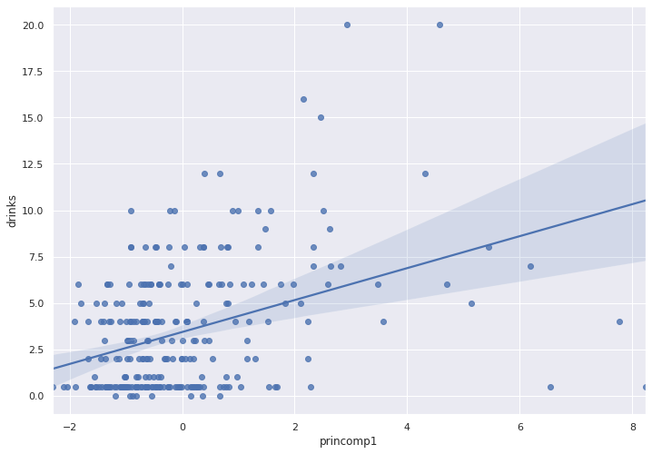
A trendline over a scatter plot indicates if we have correlation.
sns.regplot(x = pca_train_features_df['princomp1'],
            y =train_labels )
The trendline does not indicate strong correlation.
Reduce Five Dimensions to Two Dimensions
A two dimension feature set allows us to graph the two Principal Components against our label (target) vector, drinks.
pca = PCA(n_components=2)
pca.fit(normalizer(train_features))
pca_train_features_df = pd.DataFrame(pca.transform(normalizer(train_features)),
                                     columns = ['princomp1','princomp2'],
                                     index=train_features.index)
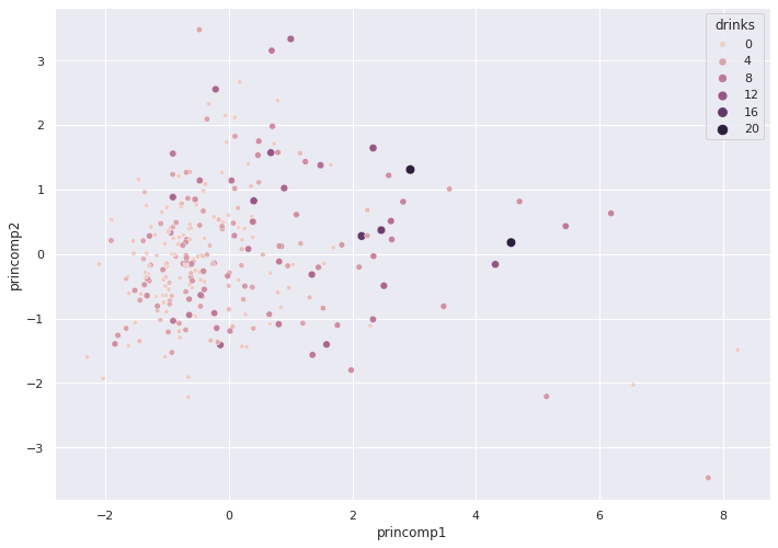
Seaborn only provides limited three dimensional plots. The following plot captures the relationship between drinks and the two Principal Components. The diameter of each circle indicates the number of drinks.
sns.scatterplot(x = pca_train_features_df['princomp1'],
                y = pca_train_features_df['princomp2'],
                hue = train_labels,
                size = train_labels)
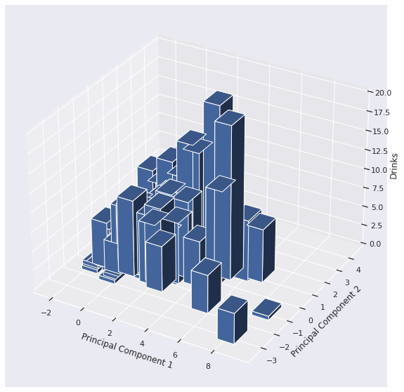
Classic MATPLOTLIB allows us to plot on three axes.
fig = plt.figure(figsize = (15, 10))
ax1 = fig.add_subplot(111, projection='3d')

x3 = pca_train_features_df['princomp1']
y3 = pca_train_features_df['princomp2']
z3 = np.zeros(len(train_labels))

dx = np.ones(len(train_labels))
dy = np.ones(len(train_labels))
dz = train_labels

ax1.bar3d(x3, y3, z3, dx, dy, dz)

ax1.set_xlabel('Principal Component 1')
ax1.set_ylabel('Principal Component 2')
ax1.set_zlabel('Drinks')

plt.show()
The height of the bars depict the number of drinks. The sloping of the bar charts indicates we may have found some slight correlation.
2. Linear Model w/ PCA
We already normalized our train dataset before we applied PCA, so we do not include the TensorFlow normalizer. We use Keras to construct and compile our new linear model.
# no need for normalizer
linear_model_pca = keras.Sequential([layers.Dense(units=1)])
linear_model_pca.compile(optimizer=tf.optimizers.Adam(learning_rate=0.1),
                         loss='mean_squared_error')
We pass the PCA-transformed, two feature data set to the model, along with the original train labels vector, that includes the number of drinks.
%%time
history = linear_model_pca.fit(
    pca_train_features_df, train_labels,
    epochs=100,
    verbose=0, #turn off loggs
    validation_split = 0.2 #validation on 20% of the training
)

CPU times: user 3.76 s, sys: 384 ms, total: 4.15 s
Wall time: 2.8 s
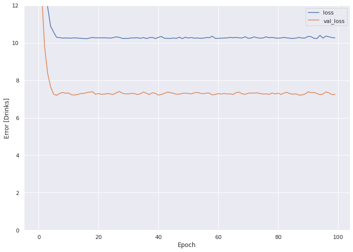
Plot the loss across each epoch for the train and validate sets.
plot_loss(history)
The train set MSE clocks in over 10, with the validate set under 8.
In order to evaluate the model with the holdout set, we first must project the five feature holdout set to two dimensional space via the PCA map matrix.
# Project test features to Principal Components
pca_test_features_df = pd.DataFrame(pca.transform(normalizer(test_features)),
                                    columns = ['princomp1','princomp2'],
                                    index=test_features.index)
The resulting holdout set now spans two (vs. five) dimensions.
print(pca_test_features_df.head())
    princomp1  princomp2
9   -1.031826  -0.390413
25  -0.900648   0.331132
28  -0.957798   1.973741
31  -0.087801  -0.594343
32  -0.242004   0.572321
How did we do?
test_results['Linear Model w/ PCA'] = (linear_model_pca.evaluate(pca_test_features_df, test_labels))**0.5
print(test_results)
3/3 [==============================] - 0s 1ms/step - loss: 9.4360
{'Linear Model': 3.217451704088136, 'DNN': 3.3038437219287813, 'Linear Model w/ PCA': 3.0718091272720853}
PCA reduces the RMSE of the Linear model from 3.2 to 3.0, pretty darn good!
3. DNN with PCA-transformed Data
We use Keras to compile a DNN and once more we do not pass a normalizer.
dnn_model_pca = keras.Sequential([
    layers.Dense(64, activation='relu'),
    layers.Dense(64, activation='relu'),
    layers.Dense(1)
  ])
dnn_model_pca.compile(loss='mean_squared_error', optimizer=tf.keras.optimizers.Adam(0.001))
We pass the PCA mapped train features to the model and set validation proportion to 20%.
%%time
history = dnn_model_pca.fit(
    pca_train_features_df, train_labels,
    epochs=100,
    verbose=0, #turn off loggs
    validation_split = 0.2 #validation on 20% of the training
)

CPU times: user 4 s, sys: 420 ms, total: 4.42 s
Wall time: 3.03 s
How do the results look?
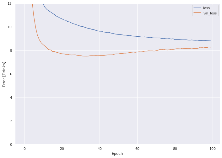
plot_loss(history)
The MSE for the validation set crosses above 8 after the 70th epoch or so.
We evaluate the DNN model with the transformed, two dimensional holdout set.
test_results['DNN w/ PCA'] = (dnn_model_pca.evaluate(pca_test_features_df, test_labels))**0.5
print(test_results)
3/3 [==============================] - 0s 1ms/step - loss: 10.0268
{'Linear Model': 3.217451704088136, 'DNN': 3.3038437219287813, 'Linear Model w/ PCA': 3.0718091272720853, 'DNN w/ PCA': 3.166514259150867}
The DNN w/ PCA reduces the RMSE from 3.3 to 3.16 vs. the original DNN.
4. Interpretation
The RMSE for the four models range from 3.07 (lowest) to 3.30 (highest). Does our model do a good job in predicting how many drinks a person consumes in a day?
To answer that, consider the formula for Root Mean Squared Error (RMSE):
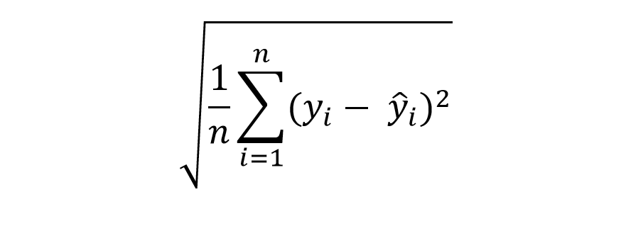
We subtract the actual value from the estimated value for each observation, square the result to remove the negative sign, sum everything up and then take the square root.
Now, assume we just guess the mean for every observation.
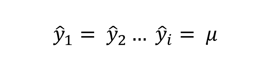
If we substitute this guess vector into our RMSE formula, we get the formula for Standard Deviation.
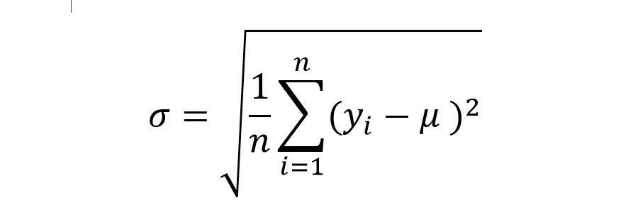
We consider, therefore, any RMSE that comes in under Standard Deviation a victory.
Take a look at the Standard Deviation of the train data set:
train_labels.std()
Out[185]:
3.4108545780181885
By this account all four models win. Keep in mind, however, in the wild most test sets will include such a high volume of data that the STD will tighten to zero.
One last thing. Assume a simple model where we just guess the mean of the train data when predicting on the holdout data. How does this simple model perform?
sq_er = (test_labels - train_labels.mean())**2
test_results['Guess Mean'] = sq_er.mean()**0.5
test_results
Out[215]:
{''Guess Mean': 3.029730661841211}
The "Guess Mean" approach out-performs all of the other models!
| Approach | Dims | RMSE |
|---|---|---|
| Guess Mean | N/A | 3.03 |
| Linear Model | 2 | 3.07 |
| Linear Model | 5 | 3.22 |
| DNN | 5 | 3.30 |
| DNN | 2 | 3.17 |
In the next blog post we will investigate ways to tune the model, from a construction and hyper-parameter tuning standpoint.
If you enjoyed this blog post, please check out these related blog posts: