Introduction
I investigate the effectiveness of a Reduced Coulomb Energy (RCE) Neural Network on the classification of the University of California, Irvine (UCI) Bupa liver disorder data set. I investigate seven (7) different versions of the data set, four (4) un-coded and three (3) binary coded (to a higher dimensional feature space) data sets applying various feature vector dimensionality reduction strategies. Finally, for all seven (7) datasets I apply a feedback-tuning algorithm. In summary, I receive a best case error rate of 20% and ambiguity of 31%, when I apply my feedback-tuning algorithm (using a learning rate of η=0.25) to the un-coded data set that reduces the feature vector dimensionality to half the original size.
Outline
- Introduction
- Background
- Why is this an important problem?
- What work has been done before?
- Brief discussion of RCE
- Benefits of RCE
- Methods
- Data
- Results
- Conclusions
- Bibliography
Background
Why is this an important problem?
A medical diagnosis contains a test pattern with features such as symptoms, patient history, and laboratory tests. The doctor uses this test pattern to diagnose, or classify the patient. Doctors and patients can benefit if the Doctor treats the diagnosis as a classification problem, and can arrive at a classification model with low error [Bojarczuk 27]. “Medical data often seem to contain a great number and uncertain or irrelevant features. How to extract enough necessary and useful diagnostic rules used to be highly depended on the clinical experience [Kahramanli 9].” I investigate if a RCE NN can extract enough necessary and useful diagnostic rules from the BUPA liver disorders data set, to reduce dependence on clinical experience, and instead put the intelligence in the pattern classification model.
What work has been done before?
Several mathematicians apply algorithms to the BUPA Liver Disorders dataset. Goncalves minimizes error to 20.31% using the Inverted Hierarchical Neuro-Fuzzy BSP System (HNFB) [Goncalves 245]. Raicharoen and Lursinsap achieve an error rate of only 18.61% using critical support vectors (CSV) [Raicharoen 2534]. Bagirov and Ugon achieve 10.14% error using their min-max separability algorithm [Bagirov 19]. Cordella classifies through genetic programming, where prototypes of the classes describe clusters of data samples and logical expressions established conditions on feature values. Cordella hits an error rate of 26.2% [Cordella 732]. Kahramanli’s Opt-aiNET algorithm lowers the error to 5.2% [Kahramanli 12]. [Kahramanli 9]. I investigate the utility of applying a RCE net method to the Bupa liver disorders dataset.
Brief discussion of RCE
Pattern classification represents distinct classes through disjoint regions formed by feature space partitioning. Most classifiers partition non-overlapping regions and map each of these to a class. In RCE networks, however, a class may have one or more regions, and regions can overlap. A RCE net contains three layers, the input, output and hidden. The input layer contains one node for each of the features, totaling the feature vector dimension. The output layer has one node for each class. In the hidden layer, each node represents a prototype. Each class connects to either one or a cluster of prototypes. A RCE net contains two modes, learning and classification. The learning mode executes feature space partitioning, adjusts connection weights between input and hidden layer, and reduces thresholds in hidden nodes to eliminate wrong activations. The classification mode makes class membership decisions based on the prototypes and their influence fields. Some regions may have multiple class affiliations, and the RCE net labels these regions “ambiguous.” [Li 847]
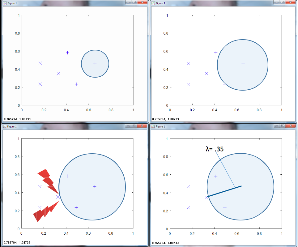
Figure 1 above illustrates part of the learning stage of an RCE net. Consider two classes of data, each with three training samples. The RCE net grows a sphere around a training point until it hits a training point of a different class. The RCE net stores this radius, λ, for that training point.
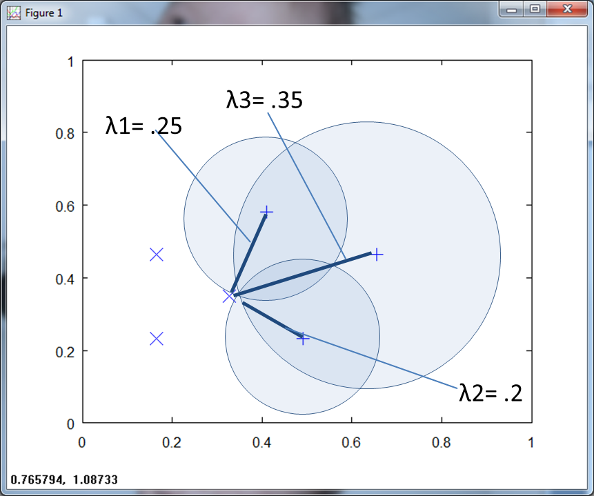
Figure 2 above shows λ for the three training points of class two (marked by a “+”).
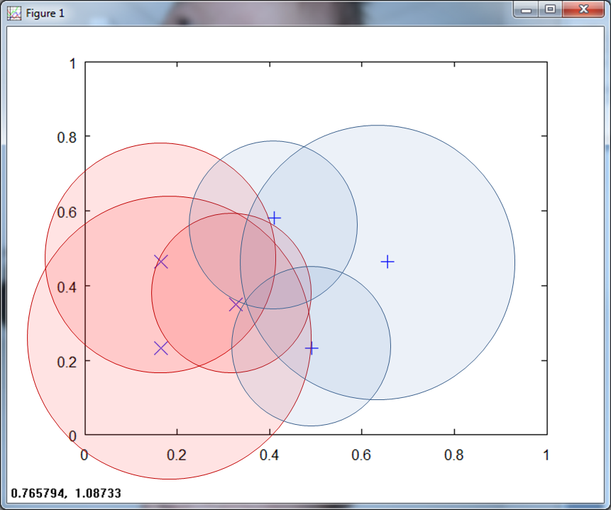
Figure 3 below depicts λ for both classes, notice how they overlap.
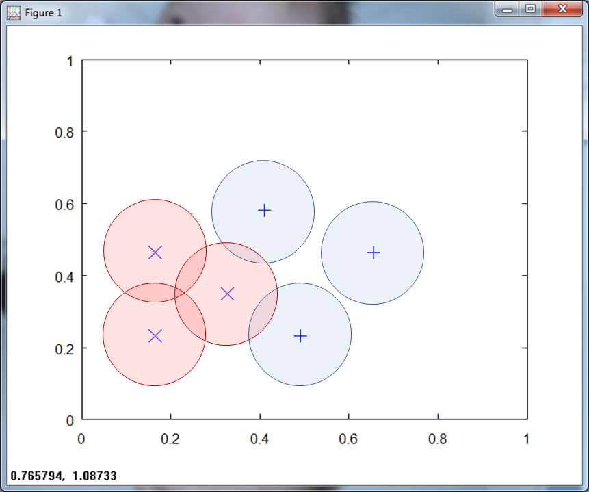
Scofield defines ambiguous regions as "point sets in the state space of a system which are labeled with multiple class affiliations. This can occur because the input space has not carried all of the features in the pattern environment, or because the pattern itself is not separable." [Scofield 5]. The RCE net reduces the overlapping region by setting a maximum λ, as shown in Figure 4 below.
The overlapping, or ambiguous regions point to regions that provide useful training points. In Figure 5 below, we show an RCE net with a large ambiguous region.
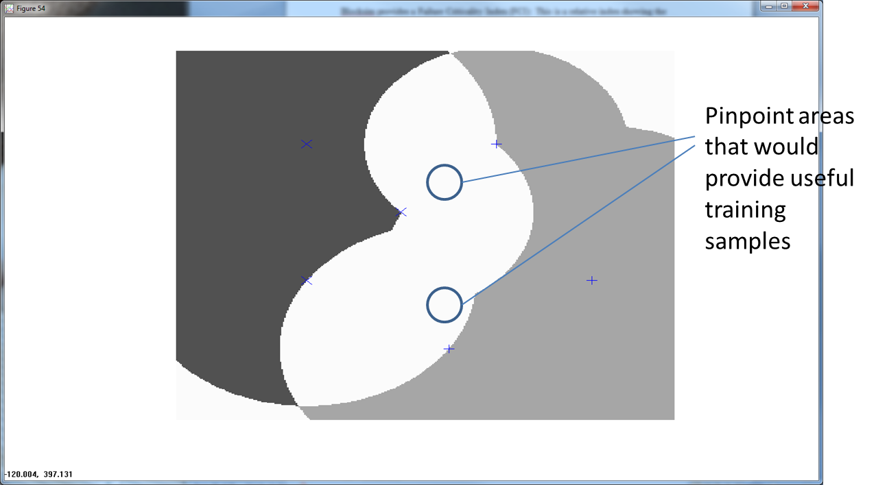
Getting training samples from this ambiguous area helps to better define the nature of the feature space.

Once the training phase completes, the RCE net classifies the test points. RCE nets belong to the family of exemplar neural net classifiers, which “perform classification based on the identity of the training examples, or exemplars, that are nearest to the input. Exemplar nodes compute the weighted Euclidean distance between inputs and node centroids [Lippmann 49].” RCE nets create hyper-spheres around training points. The related hidden layer nodes have “high outputs only if the input is within a given radius of the node’s centroid. Otherwise, node outputs are low. The classification decision is the label attached to the nodes with high outputs [Lippmann 51].” The RCE net classifies a region ambiguous in the case of no outputs or outputs from multiple classes.
Benefits of RCE
Lippmann summarizes the benefits of RCE:
This classifier is similar to a k-nearest neighbor classifier in that it adapts rapidly over time, but it typically requires many fewer exemplar nodes than a nearest neighbor classifier. During adaptation, more nodes are recruited to generate more complex decision regions, and the size of hyper-spheres formed by existing nodes is modified. Theoretical analyses and experiments with RCE classifiers demonstrate that they can form complex decision regions rapidly. Experiments also demonstrated that they can be trained to solve Boolean mapping problems such as the symmetry and multiplexer problems more than an order of magnitude faster than back-propagation classifiers. Finally, classifiers such as the RCE classifier require less memory than k-nearest-neighbor classifiers but adapt classifier structure over time using simple adaptation rules that recruit new nodes to match the complexity of the classifier to that of the training data" [Lippmann 51]
Li writes that RCE nets perform rapid learning of class regions that are, complex, non-linear and disjoint. Li also writes “RCE net has the advantage of fast learning, unlimited memory capacity, and no local minima problem” [Li 846].
Methods
I solve the problem by creating a family of MatLab/ Octave functions from the ground up, identifying the key features and then running the reduced data set through my algorithms (See Appendix). I then create a feedback approach, and identify the ground rules that yield the lowest error. If interested, you can download my Octave code from GitHub here.
Inappropriate normalization presents the first roadblock in my investigation. Normalizing between zero and one causes otherwise distinct training points from different classes to have the same magnitude. For most classification algorithms, this creates “built-in error.” For RCE nets, this results in “built-in ambiguity.” I depict this in Figure 7 below.
In addition, normalizing on a per pattern basis yields the greatest error and ambiguity. Normalizing over a class yields the next greatest error/ambiguity. Normalizing over all samples yields the lowest error, when normalizing between -1 and 1.
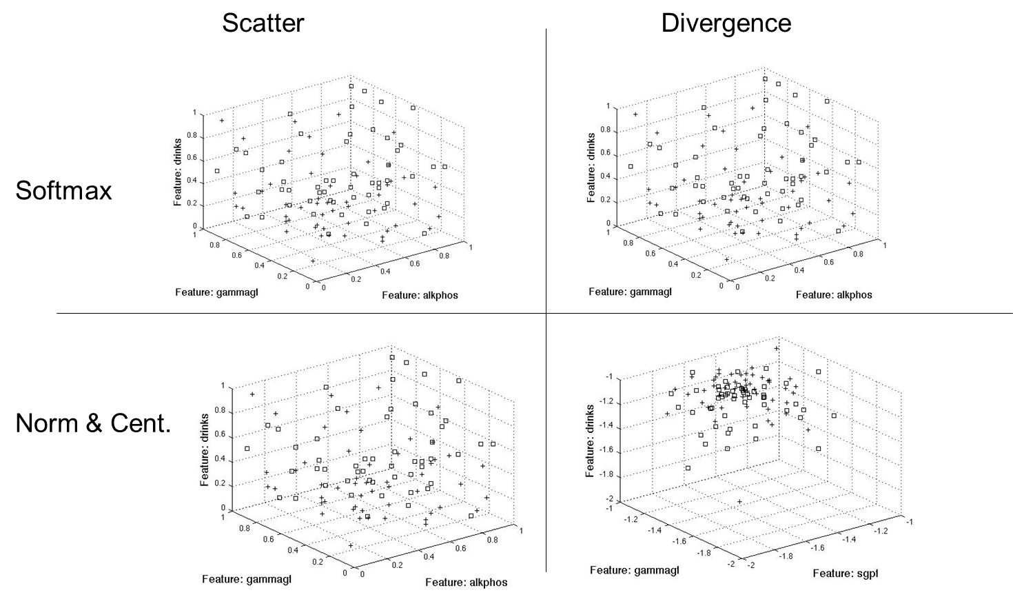
In terms of feature reduction, I use several methods, including Fisher’s discriminant ratio, divergence, Bhattacharyya distance and scatter matrices to select feature subsets.
I also run a series of analysis on binary coded Bupa data, increasing the feature dimension. For example, I take the “mcv” feature and map it into five dimensions. For mcv, I create five categories, for the ranges [0,64),[65 85),[85,90),[90,95),[95,200]. The value mcv=77 for example, mapps to the five dimensional vector [0 1 0 0 0]. The value 92 becomes [0 0 0 1 0]. This creates four new input nodes for mcv, and four of the five are always zero for any given value of mcv. I perform similar binary mapping for all the features in the BUPA data set, increasing the feature dimension from six to thirty-three (See appendix). [Kahramanli 9]
Li presents two training approaches. The first approach reduces the threshold λ of a hidden node “such that the wrong activations of this node is eliminated. This process occurs when an input pattern activates some hidden nodes which are not committed to the same class as the input pattern [Li 848].” My feedback approach uses his second approach that tunes the weights between the input and hidden nodes. The RCE net commits each hidden node to an output node of one class. If the net cannot correctly classify a known exemplar, “change weights between input nodes & hidden nodes until you activate this node [Li 848].” We must take care in changing the input to hidden weights of an exemplar classifier, since it “brings forth the potential of a training procedure whose error criterion is non-convergent [Hudak 853].” The nature of an exemplar classifier is such that changing the weights to one hidden node in order to activate it may throw off the balance of the system, and cause other patterns to become incorrectly classified.
Data
I download the BUPA liver disorders database from the University of California, Irvine (UCI) machine learning repository. The BUPA data has six features and two classes (one for alcohol related liver disorder, and one for alcohol unrelated liver disorder). BUPA features include “mean corpuscular volume (mcv),” half-pint equivalents of alcohol per day (drinks) and four chemical markers: (1) alkaline phosphotase (alkphos) (2) alamine aminotransferase (sgpt) (3) aspartate aminotransferase (sgot) and (4) gamma-glutamyl transpeptidase (gammagt). Using Fisher discriminant, Scatter Matrices, Divergence and Bhattacharyya distance methods, I pare down the feature space to candidate feature spaces. Lippmann writes, "features should contain information required to distinguish between classes, be insensitive to irrelevant variability in the input, and also be limited in number to permit efficient computation of discriminant functions and to limit the amount of training data required" [Lippmann 47]
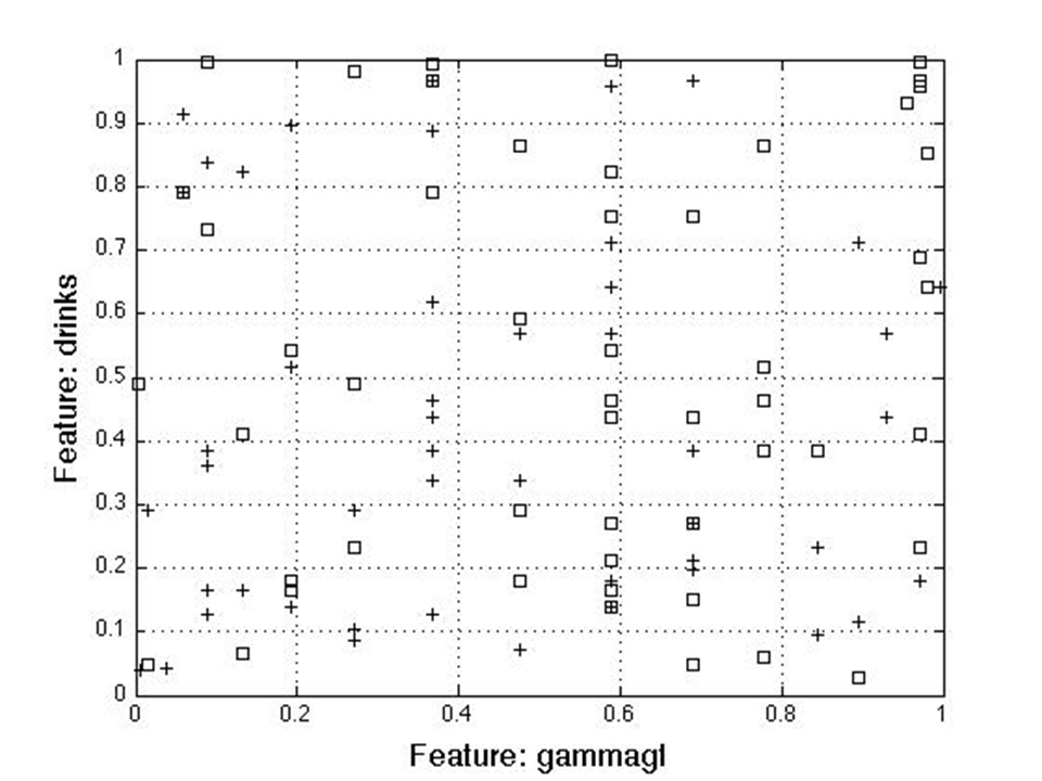
In summary, all methods picked parameters [2 5] for the two feature case, [2 5 6] for the three feature case, [2 3 5 6] for four features and [2 3 4 5 6] for five features. For the coded data, the methods selected [19 20 21 23 29] for five features, [4 9 10 14 16 18 25 28 29 30] for ten and [1 2 3 4 7 9 10 16 19 21 25 28 29 31]. This shows certain features correlate more with a class when they are coded to a certain range. The following figures (Figure 8 & Figure 9) show two (2) and three (3) feature plots:
Results
In general, coding the data does not give us any gain, either in the ‘feedback-tuned” case or the “non-feedback-tuned” RCE net case. All un-coded strategies yield lower error and ambiguity than the coded strategies, with one exception (when feedback tuned, the fifteen (15) feature coded data set yields lower error and ambiguity than the five (5) feature un-coded data set). In all cases (coded and un-coded), however, paring the feature space down yields less error than using all features, with one exception. For feedback tuning, the coded “all features” feature vector performs better than the coded ten (10) feature vector.
Using no feedback, the results follow:
- 4 Features, Un-coded: 22% error, 40% ambiguity
- 5 Features, Un-coded: 18% error, 49% ambiguity
- 3 Features Un-coded: 22% error, 45% ambiguity
- All Features Un-coded: 19% error, 49% ambiguity
- 15 Features Coded: 38% error, 40% ambiguity
- 10 Feats Coded: 31% error, 48% ambiguity
- All Features Coded: 44% error, 42% ambiguity
Using “feedback-tuning,” the three (3) feature un-coded data set yields the lowest error and ambiguity. For coded data, fifteen parameters yield the lowest error and ambiguity. Due to the delicate nature of tuning in an exemplar neural net, feedback tuning efficiency relies heavily on the learning rate. In my analysis I iterate different learning rate values (η) ranging from 0.05 to 1.0, with a step of 0.05. For each case (coded/un-coded and different feature vector dimensions), I iterate 200 times and select the lowest error/ ambiguity. In the list below, I show η that yields the lowest error/ ambiguity.
- 3 Feats Un-coded, η=0.25 20% error, 31% ambiguity
- All Feats Un-coded, η=0.10 18% error, 35% ambiguity
- 4 Feats Un-coded, η=0.15 17% error, 40% ambiguity
- 15 Feats Coded, η=0.25 33% error, 25% ambiguity
- 5 Feats Un-coded, η=0.50 17% error, 42% ambiguity
- All Feats Coded, η=0.30 36% error, 24% ambiguity
- 10 Feats Coded, η=0.70 23% error, 39% ambiguity
Not surprisingly, feedback tuning yields lower error/ambiguity than the non-feedback-tuned case, with one exception. The non-feedback-tuned four feature un-coded method actually yields lower error/ ambiguity than the feedback-tuned ten (10) feature coded method. The coded ten (10) feature method produces the worst results, which indicates poor feature selection, since the coded five (5) feature method performs better in all cases.
Now let’s look at the usefulness of my feedback strategy. The table below shows the gain (or reduction in error/ambiguity).
| Approach | Reduction in Error | Reduction in Ambiguity | Error (Gain) | Ambiguity (Gain) |
|---|---|---|---|---|
| Coded All Feats | 18.10% | 42.90% | -0.87 dB | -2.43 dB |
| Coded 15 Feats | 13.20% | 37.50% | -0.61 dB | -2.04 dB |
| Coded 10 Feats | 25.80% | 18.80% | -1.3 dB | -0.90 dB |
| Un-coded 3 Feats | 9.10% | 31.10% | -0.41 dB | -1.62 dB |
| Un-coded All Feats | 5.30% | 28.60% | -0.23 dB | -1.46 dB |
| Un-coded 4 Feats | 22.80% | 0.00% | -1.12 dB | 0.00 dB |
| Un-coded 5 Feats | 5.60% | 14.30% | -0.25 dB | -0.67 dB |
In all cases, my tuning algorithm helps reduce the error and/or ambiguity. My tuning algorithm produces the most gain for the inferior performing “coded” data set.
Conclusion
Lippmann and Hudak criticize RCE nets. Lippmann writes, RCE nets “may require large amounts of memory and computation time [Lippmann 49].” Hudak writes, “Viewing RCE as an incremental nearest-neighbor classifier with hyper-spheres lads to the conclusion that the hyper-spheres are not positively contributing to the performance of the classifier. At best their presence is ineffectual, but their management during training entails a computational cost that is not justified by these findings [Hudak 852].”
I experience a “computational cost” during management of the RCE net training. Iterating through 20 candidate values of η, and then iterating 200 learning steps for each takes tens of minutes. Once I identify the proper weight tuning for the data, however, classification occurs in real time. RCE does have benefits, due to the ambiguity. Even Hudak writes, “hyper-spherical classifiers can recognize patterns from an unknown class as not belonging to any class known to the classifier. If true, this would be an advantage over the nearest-neighbor classifier [Hudak 853].”
In conclusion, binary coding does not help reduce error/ ambiguity. Reducing the feature set on the un-coded data reduces error/ ambiguity. My feedback-tuning algorithm, while computationally expensive, reduces error/ ambiguity in all cases. The feedback-tuning algorithm yields the greatest gain on the poorer-performing coded data set. The best case scenario shows reducing the un-coded feature vector to half its dimension using the features “alkaline phosphotase, “gamma-glutamyl transpeptidase” and “number of half-pint equivalents of alcoholic beverages drunk per day” and feedback tuning using a learning rate of η=.25. This yields an error of 20%, and an ambiguity of 31%.
If you enjoyed this blog post, please check out these related blog posts:
- Exploratory Factor Analysis (EFA) Workflow and Interpretation
- EFA - The Math and Algorithms
- Probabalistic Parzen Neural Networks (PNN) with cartoons
- Vision model w/ FAST AI
- Vision model w/ Google AutoML
- Google AutoML Tables Beta
Bibliography
Bagirov, A.M., Ugon, J. “Supervised Data Classification via Max-min Separability.” Mathematical Modeling of Bio-systems Springer Berlin Heidelberg, 2008: 1-23
Bojarczuk, C.C., Lopes, H.S., Freitas, A.A. and Michalkiewicz, E. L. “A constrained-syntax genetic programming system for discovering classification rules: application to medical data sets.” Artificial Intelligence in Medicine 2004:27-48
Cooper, Leon N. “A Neural Model for Category Learning.” Center for Neural Science and Department of Physics, Brown University Providence, R.I. 1982
Cordella, L.P., De Stefano, C., Fontanella, F. “A Novel Genetic Programming Based Approach for Classification Problems.” Lecture Notes in Computer Science, Image Analysis and Processing ICIAP 2005: 727-734
Goncalves, L.B., Vellasco, M.M., Cavalcanti, M.A., Pacheco M.A. “Inverted Hierarchical Neuro-Fuzzy BSP System:A Novel Neuro-Fuzzy Model for Pattern Classification and Rule Extraction in Databases.” IEEE Transactions On Systems, Man And Cybernetics Part C: Applications And Reviews 2006: 236-248
Hudak M.J. “RCE Networks: An Experimental Investigation.” Neural Networks, 1991., IJCNN-91-Seattle International Joint Conference on Jul. 1991: 849-854
Kahramanli, Humar, Allahverdi, Novruz “Mining Classification Rules for Liver Disorders.” International Journal of Mathematics and computers in simulation Issue 1, Volume 3: 2009
Li, Wei “Invariant Object Recognition Based on a Neural Network of Cascaded RCE nets.” Neural Networks, 1990., 1990 IJCNN International Joint Conference on Jun 1990:17-21
Lippmann, Richard P. “Pattern Classification Using Neural Networks.” IEEE Communications Magazine Nov. 1989
Raicharoen, T., Lursinsap, C. “Critical Support Vector Machine Without Kernel Function.” Neural information Processing, 9th International Conference on (ICONIPOZ) 2002: 2532-2536
Roan, Sing-Ming “Fuzzy RCE Neural Network.” Fuzzy Systems, 1993., Second IEEE International Conference on 1993:629-634
Scofield, Christopher L. “Pattern class degeneracy in an unrestricted storage density memory.” Nestor, Inc. Providence, RI. 1988