Caution! Math Ahead!
For the Math-phobic, I explain how I crunch the test results in a math-free, simple and focused blog post here.
I use math here, so this may be your last chance to escape! Still with me? Excellent!
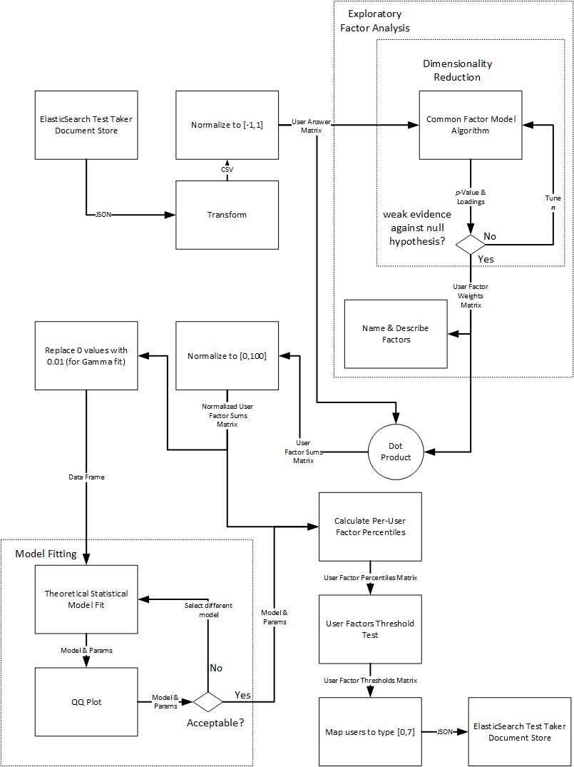
The bullets below outline the steps we take. A flow diagram follows.
- Transform Elasticsearch Database to Comma Separated Variables (CSV)
- Load into R
- Normalize data
- Exploratory Factor Analysis (EFA)
- Dimensionality Reduction (Iterate on n)
- Plot Data on Graphs
- Identify Factor Names
- Isolate Factor Weight Matrix
- Dot Product Answer Matrix with Weight Matrix
- Fit Factor Sums matrix Theoretical Models
- Plot Data
- Guess Distribution
- Fit, Graph, QQ-Plot
 Extract and Transform
I chose a NoSQL Elasticsearch document store (DataBase) to hold all of the test results, metadata and identity information. In addition to private search services (i.e. auto-completion, 'did you mean?', etc.) Elasticsearch provides (massive) scalability and integration with a robust web based GUI named Kibana. Kibana provides trend plots, pie graphs, keyword searches and a host of other features.
I need to extract data from the NoSQL document store and translate it into a structured format for R. I use the excellent Elasticsearch Domain Specific Language (DSL) python library to do just that.
As I mentioned in HOWTO-1, I must first serialize the data to JSON, in order to use the Amazon IAM serivce with the Amazon Elasticsearch service. When I roll up my sleeves and dive in, I notice the (trivial) Elasticsearch DSL "scan" method requires a low-level Elasticsearch client connection object to perform.
In order to use REST/JSON calls, therefore, I need to scan "by hand." The official Elasticsearch documents point us to the low level elasticsearch-py libraries but since elasticsearch-dsl extends these, they do not help with our problem of needing to serialize to JSON and pass via an extended AWSAuthConnection object.
To scroll by hand, I first request the Elasticsearch API to set the search type to "scan" with a scroll duration of ten minutes. Elasticsearch responds with a scroll ID. I use the scroll ID to request the first batch of documents, and Elasticsearch responds with the documents and the current scroll_id (it may update). I then iterate until the process finishes.
while True:
r = client.make_request(method='GET',path='/_search/scroll',data=json.loads(r.read())['_scroll_id'],params={"scroll":"10m"})
if len(json.loads(r.read())['hits']['hits']) > 0:
#...process the documents
else:
break
HOT TIP: Dump an Entire Document Store
If you connect to your ES AWS service via an IAM role (AWSAuthConnection) then
(1) Make a scan request to turn off sorting
(2) Set an appropriate scroll duration (10 minutes)
(3) Iterate through all of the documents with a scroll request
(a) On each iteration, pass the current scroll_id(If you connect to your AWS service via IP whitelisting then use your search object's scan method, e.g. s.scan())
Elasticsearch returns all of the documents in a schemaless JSON format.
For example:
{
"_index" : "pilot",
"_type" : "test",
"_id" : "AVHfVLNTHootPMn5yhhf",
"_version" : 5,
"found" : true,
"_source":{"q47":"y","q2":"y","q6":"y","q33":"y","q25":"y"}
}
We need to transform the schema-less responses into something structured. With Python, we can translate the dictionary {"q47":"y","q2":"y","q6":"y","q33":"y","q25":"y"} into a table format for R to read.
Note the arbitrary placement of the questions in the JSON response. We need simple logic to cycle through all fifty questions (q0, q1 ... g49) and test if they reside in the response. We could use a case statement with fifty individual tests but instead I decided to use arrays. I create a simple list, "q" with string names for each question. I then create an array, "scorecard" with fifty zeros. If the while loop discovers a match for a question, "q25" for example, it places a one (1) in that list position of scorecard. At the end I receive a table of results, one row per document, and a positional on/off for each "yes" in that document.
The dump script follows:
The script transforms...
{
"_index" : "pilot",
"_type" : "test",
"_id" : "AVHfVLNTHootPMn5yhhf",
"_version" : 5,
"found" : true,
"_source":{"q47":"y","q2":"y","q6":"y","q33":"y","q25":"y"}
}
...into one row.
AVHfVLNTHootPMn5yhhf,0,0,1,0,0,0,1,0,0,0,0,0,0,0,0,0,0,0,0,0,0,0,0,0,0,1,0,0,0,0,0,0,0,1,0,0,0,0,0,0,0,0,0,0,0,0,0,1,0,0
Exploratory Factor Analysis
James H. Steiger writes an excellent white paper on using R for EFA titled "Exploratory Factor Analysis With R." I tried out several of the R libriaries to include principal and factor.pa in the psych and princomp and factanal in stats.
The princomp library got me really excited at first because all of the vectors made perfect sense (in terms of groupings the questions by "yes's" ). When I applied the weight matrix to the initial answer matrix I saw that 80% of the test takers fell into the first component. This concerned me at first until I realized that the first component held most of the varience and that raw PCA would not be the appropriate tool to separate test takers into roughly equal groupings.
The hilariously named factanal (huh huh Bevis)library accomodated my use case. I used the common factor analysis approach (vs. component analysis) which fits via Maximum Likelyhood and rotated with varimax.
I first loaded the data and normalized my data set to the range of [-1,1].
bdpt = read.csv('data.csv',stringsAsFactors = FALSE)

# Get rid of the ID's
bd = bdpt[2:51]

# Uncomment to change zeros to negative ones
bd[ bd == 0] <- -1

# Uncomment to sample
ind <- sample(10000,1000)
bd <- bd[ind,]
I fit with Maximum Likelyhood, select three (3) dimensions and rotate with varimax.
fit <- factanal(bd, 3, rotation="varimax")
We can look at the loadings for each factor.
Loadings:
Factor1 Factor2 Factor3
tire 0.114 0.214
rich 0.231 0.222
dangerous 0.257 0.165
fame 0.172 0.169
hair 0.200 0.168 0.199
bet
taxes 0.143 0.286
execute 0.141 0.303
castle 0.167 0.105
losers 0.139 0.290
pretty_women 0.796
pretty_men 0.676
vhs 0.184 0.186
punch 0.362 0.164 0.109
jerkface 0.380 0.151
facebook 0.128 0.113
champion 0.439
God -0.300 0.237
speed
advice 0.291
mouse 0.229 0.169
drunk 0.406 0.165
kleeb 0.267
gravitate 0.224 0.259 0.118
no_plan 0.309 0.222
drugs 0.445
fan 0.136
work_hard 0.304 0.124
potential
intelligence 0.210 0.218
wait_food 0.298
bossy 0.127 0.105
world_against 0.264 0.156
suffer_evil 0.409
trust_cops -0.245 0.276
learning 0.408
cult 0.383
naked 0.328 0.135
door 0.159 0.167
grass 0.158 0.184 0.131
paycheck 0.242
fashion 0.155 0.266
locks 0.204
love 0.229 0.110
dogs 0.362
baby_corner 0.178 0.253
listen 0.157
transit 0.124 0.333
motorcycle
driver 0.154 0.103 0.134
The chart shows that "being drunk in public" and "not believing in God" correlates strongly with factor 1, "championing others" and "suffering evil vs. being evil" correlates with factor 2, and "men/women should be pretty" highly correlates with factor 3. I named these factors "hellraiser," "boy scout" and "celebrity."
The code that follows shows the relative weights of each "question" for each factor. I provide 2d and 3d graphs. For more detail, click here.
# #################
# # Graph Factors #
# # in 2 and 3d #
# #################
layout(matrix(c(1,1,1,2,3,4), 2, 3, byrow = TRUE))

pcolor <- apply(fit$loadings,1,which.max)
pcolor[pcolor==1] <- "red"
pcolor[pcolor==2] <- "blue"
pcolor[pcolor==3] <- "darkgreen"
s3d <- scatterplot3d(fit$loadings,color=pcolor,pch=19,type="h", lty.hplot=2,scale=3,angle=55,xlab="Hellraiser",ylab="Boy Scout",zlab="Celebrity")
s3d.xyz <- s3d$xyz.convert(fit$loadings)
text(s3d.xyz$x, s3d.xyz$y, labels=row.names(fit$loadings), cex=.7, pos=4)
legend("topleft", inset=.05, bty="n", cex=.5, title="Factor Assignment", c("Hellraiser", "Boy Scout", "Celebrity"), fill=c("red", "blue", "darkgreen"))

load <- fit$loadings[,1:2]
plot(load,type="n",xlab='Hellraiser',ylab='Boy Scout')
title('Hellraiser vs. Boy Scout')
abline(v=0,h=0,lty=2)
text(load,labels=names(bd),cex=.7)

load <- fit$loadings[,c(1,3)]
plot(load,type="n",xlab='Hellraiser',ylab='Celebrity')
title('Hellraiser vs. Celebrity')
abline(v=0,h=0,lty=2)
text(load,labels=names(bd),cex=.7)

load <- fit$loadings[,2:3]
plot(load,type="n",xlab='Boy Scout',ylab='Celebrity')
title('Boy Scout vs. Celebrity')
abline(v=0,h=0,lty=2)
text(load,labels=names(bd),cex=.7)
#
Crunch the Numbers
For each test taker, I tally up their total factor weights based on they answer each question. To process the data, I perform a simple dot product of the "User Answer Matrix" and the "User Factor Weight" matrix, which yields a "User Factor Sums Matrix." I then normalize the "User Factor Sums Matrix" and pull out zero values in order to try certain theoretical fits (such as Gamma).
########################
# The number crunching #
########################

# Convert loadings to a weight matrix
pca <- apply(fit$loadings,2,function(x) x)

# Dot product of answers with the weight matrix
# to get factor sums for each test taker
answer <- as.matrix(bd) %*% as.matrix(pca)

# Normalize the test taker's factor sums
# between 0 and 100
norm_answers <- sapply(seq_len(3),
function(i) round((answer[,i] - min(answer[,i]))*100/(max(answer[,i]) - min(answer[,i])),2))

# Get rid of the Zero values
# so we can fit to a Gamma
norm_answers[norm_answers == 0] <- 0.01
Each user has a weight sum for each factor. I take these data points and try to fit them to a theoretical model. I use the Gamma function to begin. The following lines fit the data and then pull out just the shape and rate parameters for each of the three fits.
# Figure out rate and scale for fit for each factor
gamma_fit <- sapply(seq_len(3), function(i) fitdistr(norm_answers[,i],"gamma"))
# Pull just shape and rate
gamma_fit <- sapply(seq_len(3), function(i) gamma_fit[,i]$estimate)
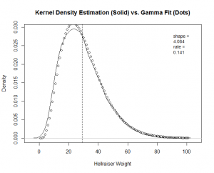
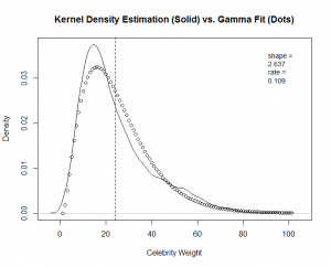
The next example shows the code for the "Hellraiser" factor. I plot a Kernel Density Estimation (KDE) of the empirical data. I then overlay points pulled from a Gamma density function with the "shape" and "rate" parameters that we found above. I show the code for "Hellraiser," and you will find the complete code at the end of this blog post.
# "Hellraiser" pdf
plot(density(norm_answers[,1]),xlab='Hellraiser Weight',main = 'Kernel Density Estimation (Solid) vs. Gamma Fit (Dots)')
abline(v=mean(norm_answers[,1]),lty=2)
legend("topright", inset=.05, bty="n", cex=.9, title=NULL, c(append("shape = ",toString(round(gamma_fit[,1][1],3))),append("rate = ",toString(round(gamma_fit[,1][2],3)))) )
par(new=T); points(dgamma(seq(0,100),shape=gamma_fit[,1][1],rate=gamma_fit[,1][2]))
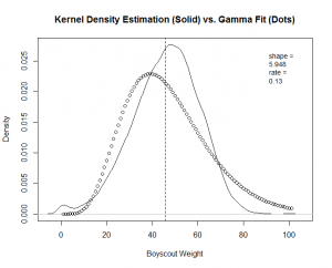
You can see a good fit for "Hellraiser" and "Celebrity," but a poor fit for "Boy Scout."
# Hellraiser
x.fit <- rgamma(n=length(norm_answers[,1]),shape=gamma_fit[,1][1],rate=gamma_fit[,1][2])
x.empirical <- norm_answers[,1]
qqplot(x.empirical,x.fit, main="Sample vs. Theoretical for Hellraiser Fit"); abline(0,1)
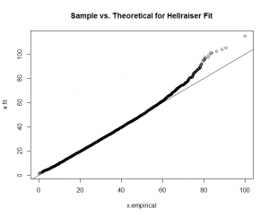
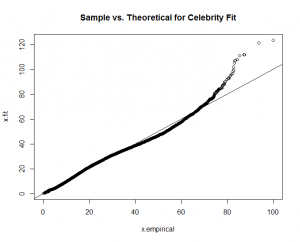
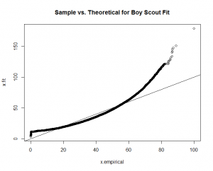
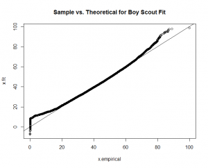
Again, good fits for all the factors except for "boy scout." With this guidance, I re-fit the "boy scout" data to a "normal" theoretical model.
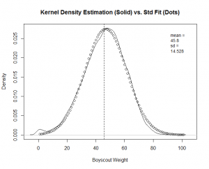
# Find mean and sd
std_boyscout_fit <- fitdistr(norm_answers[,2],"normal")
The calculation produces a much better fit, as witnessed by the new "Boy Scout" overlay plot and QQ-Plot.
We know the factor weight sums for each user. We then use our new density functions to find out where they stand compared to the other users. We give them a percentile and send each user sum weight vector to the appropriate theoretical model, with the appropriate density function parameters.
# Convert the normalized weights to percentile
# based on our fit model distributions
percentiles <- round(
sapply(seq_len(3),function(i) pgamma(norm_answers[,i],shape=gamma_fit[,i][1],rate=gamma_fit[,i][2])),2)

# Replace the gamma fit for Boy Scout
# with the Standard
percentiles[,2] <- round(pnorm(norm_answers[,2],mean = std_boyscout_fit$estimate[1], sd = std_boyscout_fit$estimate[2]),2)
``

We append the percentiles to the results matrix and execute simple "on/off" logic. If the user lies in the greater than fiftieth percentile, we turn that factor on. The simple binary logic then gives us eight types. We assign a type to each user by performing conversion from binary to decimal. A dot product between the three dimensional factor vector and the vector [1,2,4] performs the conversion.


```R
# For all test takers, set all values below mean to zero (per factor)
percentiles[percentiles < 0.5] <- 0

# Set all values above mean to one (per factor)
percentiles[percentiles != 0 ] <- 1

# Map each test taker to one of seven classes based on their on/off values for each factor
classifications <- apply(percentiles,1,function(x) as.vector(x) %*% as.vector(c(1,2,4)))
When you take the test (after I batch process), you will receive you classification and percentiles for each of the three factors.