Model optimization on traditional Artificial Intelligence and Machine Learning (AI/ML) platforms requires considerable Data Architect expertise and judgement. These ML platforms require the Architect to choose from dozens of available training algorithms. The platforms also provide a host of hyper-parameter knobs and switches for the Architect to tune. The deluge of choice requires the Architect to iterate on both algorithm selection and hyper-parameter values, a time consuming proposition.
AutoML services democratize model development via no-code, graphical user interface (GUI) based optimization services. We discuss the Google Compute Platform's (GCP) AutoML Vision service in an earlier blog post. In this blog post we discuss the GCP AutoML Tables Beta service.
The Data Set
The GCP AutoML Tables Beta service requires structured, Data Frame encoded data. To test drive the service, we use the BUPA Liver Disorders data set. For a refresher on the BUPA Liver Disorders data set, please right click and open one or more of the following blog posts in a new tab (or set of tabs):
- Applying a Reduced Columb Energy (RCE) Neural Network to the BUPA Liver Disorders Data Set
- A Graphical introduction to Probabilistic Neural Networks (PNN)
- Refactoring Matlab Code to R Tidyverse
- Fast and Easy Regression with Keras and TensorFlow 2.3 (Part 1 - Data Exploration & First Models)
- Fast and Easy Regression with Keras and TensorFlow 2.3 (Part 2 - Dimensionality Reduction)
In the latter two blog posts, we crunch the BUPA Liver Disorders data set in TensorFlow via Neural Net and Linear Regression Models and reduce model over-fit via dimensionality reduction.
The following table captures the results of our model iteration:
| Approach | Dims | RMSE |
|---|---|---|
| Guess Mean | N/A | 3.03 |
| Linear Model | 2 | 3.07 |
| Linear Model | 5 | 3.22 |
| DNN | 5 | 3.30 |
| DNN | 2 | 3.17 |
NOTE: Our TensorFlow 2.3 and Keras 2.3 investigations use the Root Mean Square Error (RMSE) success metric for model tuning
We iterate over the different model scenarios and draw the interesting conclusion that simply guessing the mean of the training data set yields the best results.
Google AutoML Beta executes a battle of the bands and iterates through dozens of algorithm choices. For each algorithm, the service tunes Hyper Parameters, to include number of layers, learning rate and number of features.
Let's see if the Google AutoML service can beat our idiotic, yet successful choose mean algorithm.
Enable GCP AutoML tables
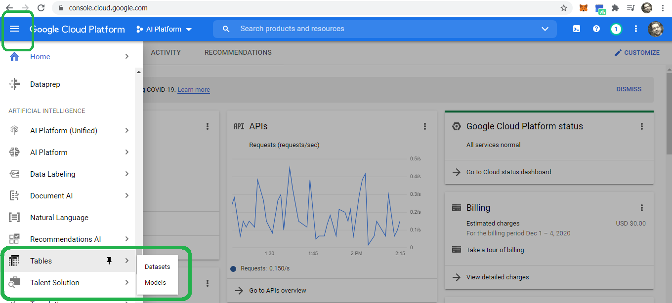
Engineers at Google call the menu selection icon the hamburger, a bit of slang that simultaneously makes me laugh and makes me hungry. Click the hamburger icon in the upper left corner and then scroll down to Artificial Intelligence and select Tables --> Datasets.
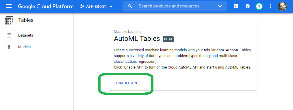
Click enable the API.
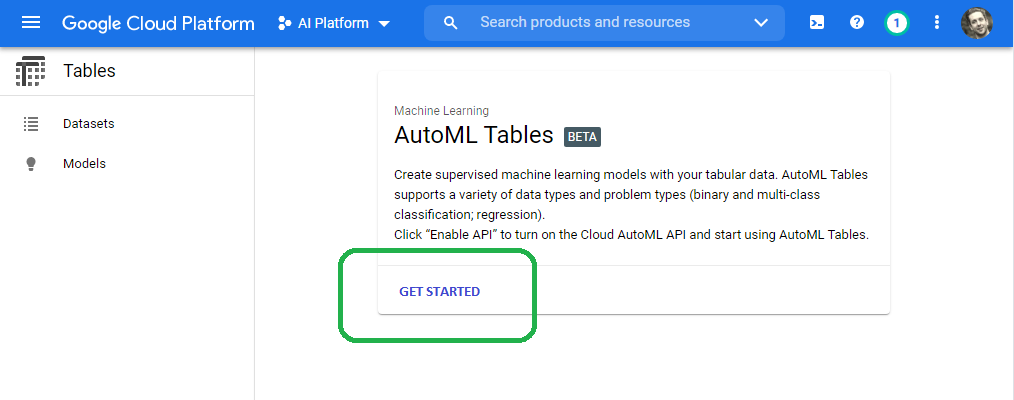
Once we enable the API, click get started.
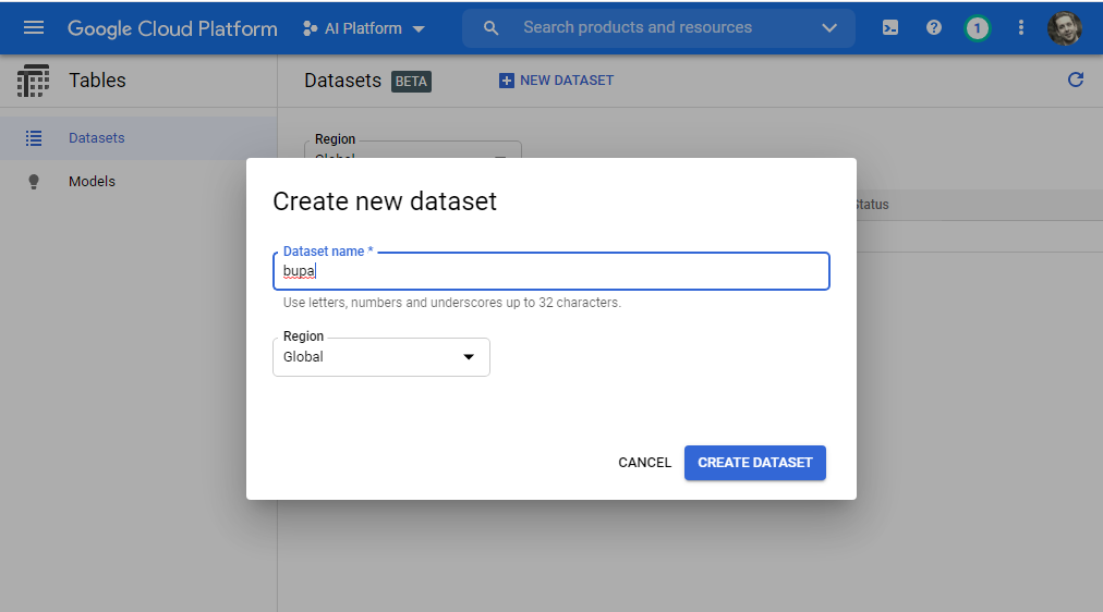
Name our dataset on the create dataset screen.
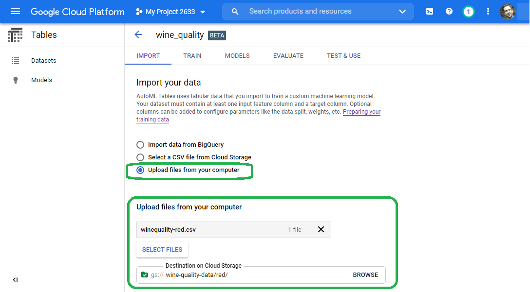
The AutoML Tables Beta service provides three vehicles for dataset import:
- Import data from BigQuery
- Select a CSV file from Cloud Storage
- Upload files from your computer
We will upload the BUPA dataset from our computer.
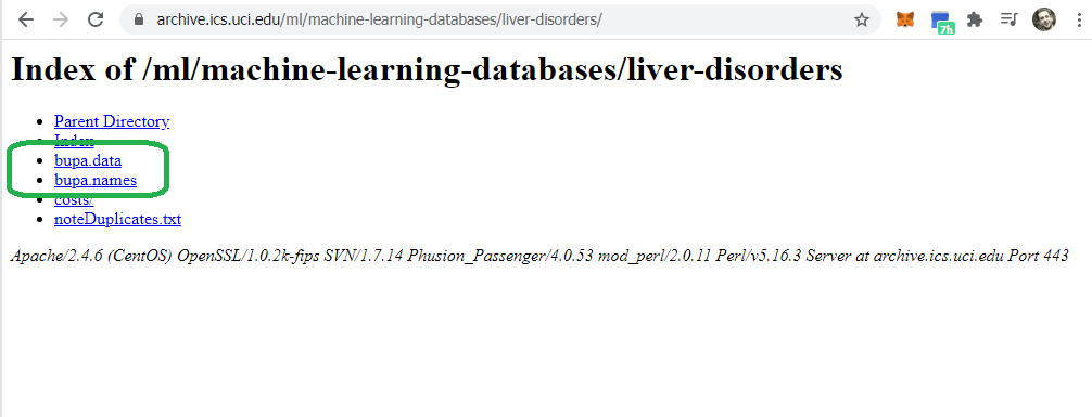
Click here to download the CSV file from USC.
USC names the file bupa.data. If we attempt to upload the file bupa.data, Google will bark.
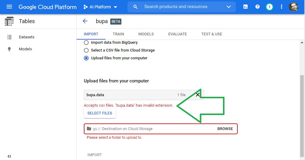
Rename our file from bupa.data to bupa.csv in order to upload the data. Click select files and then click the bupa.csv file.
If needed, create a bucket to store the model and metadata. Click browse and then select the Swiss lunch pail (my terminology, not Google's).
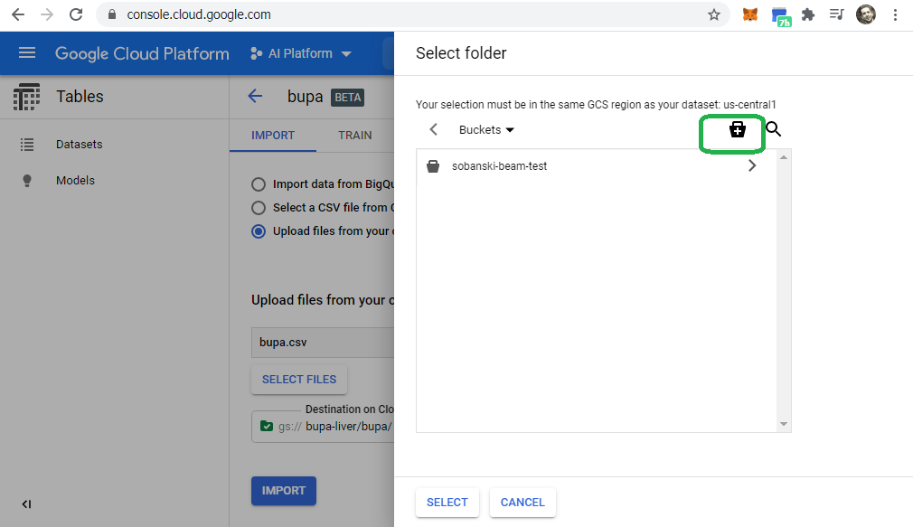
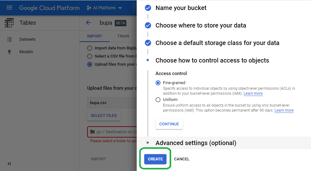
Cycle through the bucket wizard and click create.
If needed, create a folder via the Swiss lunch pail.
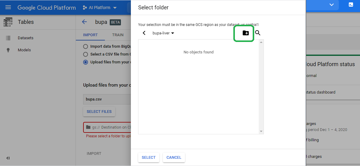
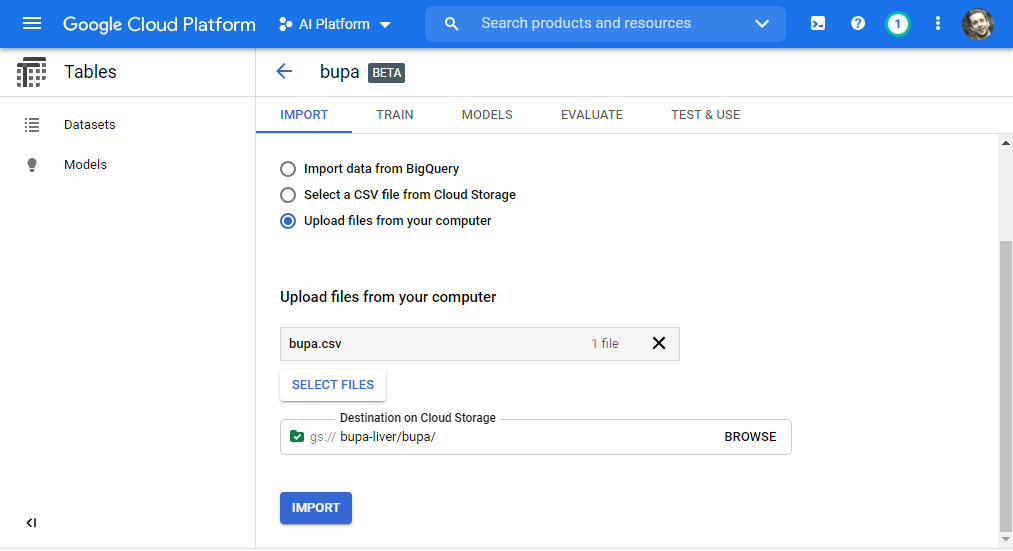
If done properly, we will see all green, and will be able to click import.
Click Import
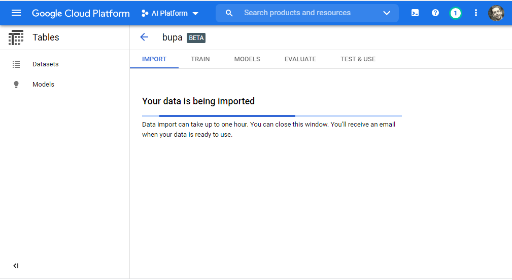
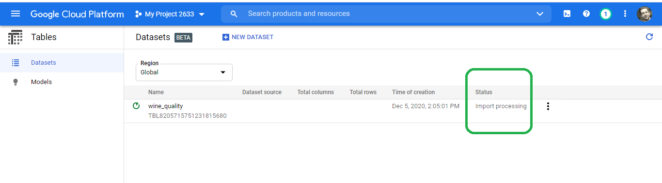
Google will import the data, a process which can take hours. We can close the window and Google will email us once they (it?) completes the import process.
After a few minutes, the import fails!
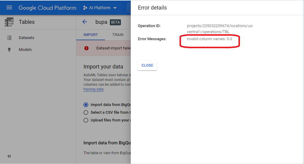
The Beta service requires a header. We hope the Alpha version will provide a friendlier UI, and provide a wizard to create a header row. Until then, we will need to add the header row by hand:
mcv,alkphos,sgpt,sgot,gammagt,drinks,selector
85,92,45,27,31,0.0,1
85,64,59,32,23,0.0,2
86,54,33,16,54,0.0,2

     <snip>

91,68,27,26,14,16.0,1
98,99,57,45,65,20.0,1
We properly wrangled the data into a form that the Google service accepts. Upload the modified bupa.csv into the import wizard and select import once more.
GCP imports the data...
...and fails once more!
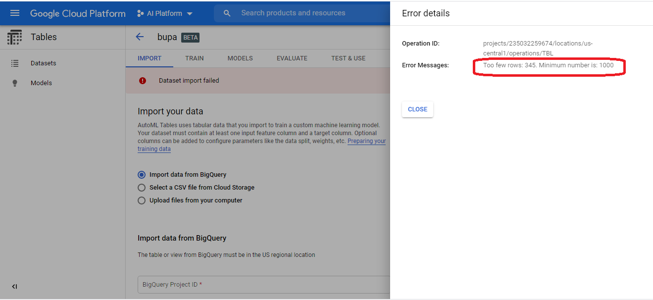
The service does not accept data sets that contain less than 1,000 rows. For this reason, we can't optimize the BUPA Liver Disorders model with Google AutoML Tables Beta, a reality that disappoints me greatly.
Imagine that you drive trucks cross-country for a living. Now imagine every morning a magical elf appears and hides your keys, steals your engine or slashes your tires. This analogy captures the daily frustration faced by professional Data Engineers!
The Beta version of the Google AutoML Tables service dashed my plans of providing a consistent machine learning narrative centered on the BUPA Liver Disorders data set. Un-cooperative software slayed my plans (and dreams) enough times in my professional career to vaccinate me against such roadblocks. With a heavy heart, I will re-group and select a new data set for us to test drive the with the AutoML Tables Beta service.
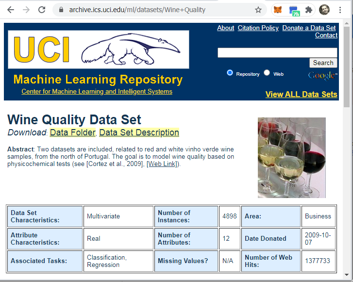
The UCI Wine Data Set
Our BUPA liver disorders TensorFlow model predicts the number of drinks that a boozer drinks each day based on biological markers. We stick with the wino theme and use the University of California Irvine (UCI) wine quality data set. The Wine Quality data set uses biological (and chemical) markers to predict the quality of wine, which the sommeliers give a score from one to ten. I would assume that Thunderbird would score low on such a scale.
Download the wine dataset from the same UCI website that hosts the BUPA data set.
We follow the method described in the BUPA TensorFlow blog post to process the data, replacing the BUPA Data Frame with the new Wine Data Frame where appropriate.
The following Python code, for example, uses the requests library to download the Wine Quality data set from the UCI website, and stuffs the data into a Pandas Data Frame.
import pandas as pd
import numpy as np
import io
import requests
url = 'https://archive.ics.uci.edu/ml/machine-learning-databases/wine-quality/winequality-red.csv'
r = requests.get(url).content
column_names = ['fixed_acidity',
'volatile_acidity',
'citric_acid',
'residual_sugar',
'chlorides',
'free_sulfur_dioxide',
'total_sulfur_dioxide',
'density',
'ph',
'sulphates',
'alcohol',
'quality']
wine_df = pd.read_csv(io.StringIO(r.decode('utf-8')),
                      sep =";",
                      header = 0,
                      names= column_names).astype(np.float32)
The table below captures the summary statistics for the wine dataset:
| feature | mean | std |
|---|---|---|
| fixed_acidity | 8.31 | 1.74 |
| volatile_acidity | 0.53 | 0.18 |
| citric_acid | 0.27 | 0.20 |
| residual_sugar | 2.52 | 1.30 |
| chlorides | 0.09 | 0.05 |
| free_sulfur_dioxide | 15.8 | 10.4 |
| total_sulfur_dioxide | 46.5 | 33.0 |
| density | 1.00 | 0.00 |
| ph | 3.31 | 0.15 |
| sulphates | 0.66 | 0.16 |
| alcohol | 10.4 | 1.08 |
| quality | 5.63 | 0.81 |
NOTE: We observe a standard deviation of 0.809201 for the target variable quality
Note the wild range swings amongst the features. We follow the same process from our BUPA model to normalize the data via TensorFlow. The following histogram records the normalized data histograms. Note that we do not normalize the target, quality.
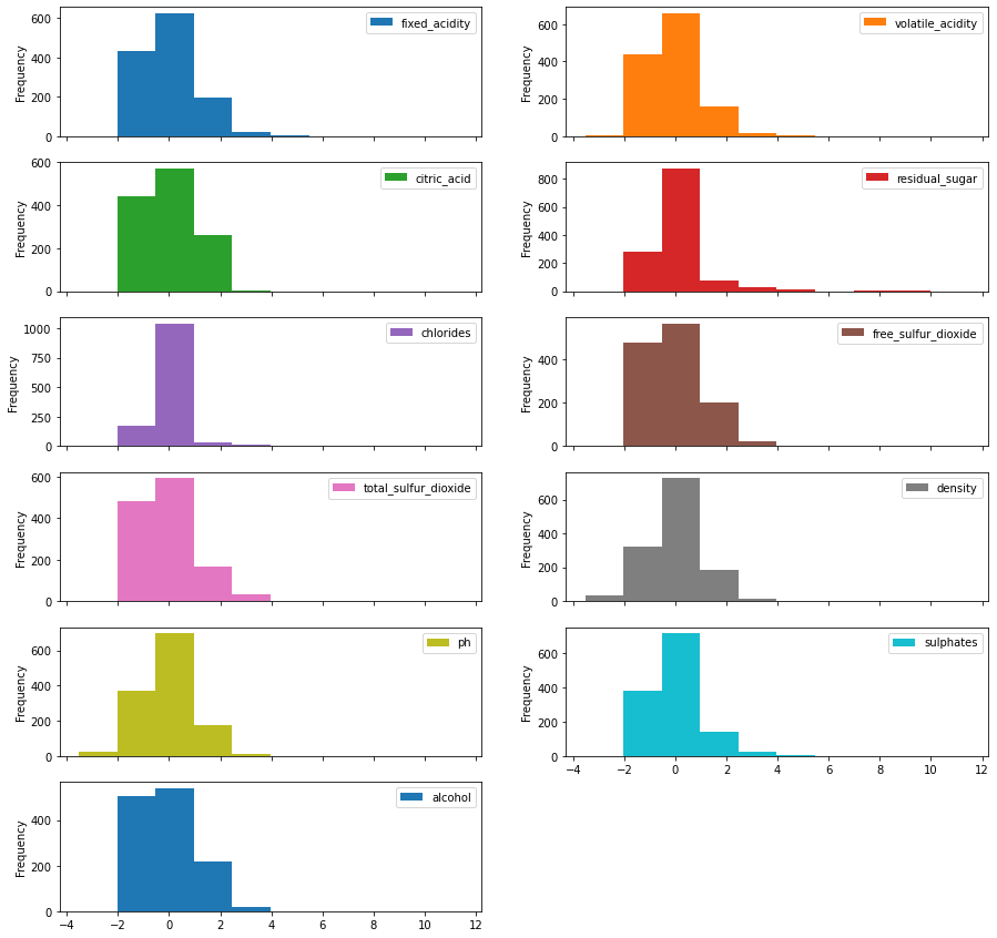
Recall that the idiotic guess mean algorithm yielded the best results for the BUPA data set. That algorithm guesses the mean of the training Data Frame for each row in the holdout (or test) Data Frame. If we apply that algorithm to the Wine Data Frame, we observe a RMSE of 0.8012159, with a RMSE greater than the standard deviation of the entire population. This result compels us to apply more advanced algorithms.
Once more, Keras provides the tools to create a linear regression model and a Dense Neural Network (DNN) model, both of which predict the quality of the wine based on the given features.
NOTE: Keras detects that we now have eleven input features, versus the five for BUPA.
dnn_model.summary()
Model: "sequential_1"
_________________________________________________________________
Layer (type)                 Output Shape              Param #
=================================================================
normalization_5 (Normalizati (None, 11)                23
_________________________________________________________________
dense_1 (Dense)              (None, 64)                768
_________________________________________________________________
dense_2 (Dense)              (None, 64)                4160
_________________________________________________________________
dense_3 (Dense)              (None, 1)                 65
=================================================================
Total params: 5,016
Trainable params: 4,993
Non-trainable params: 23
The normalized training set yields the following results:
| Approach | Dims | RMSE |
|---|---|---|
| DNN | 11 | 0.648 |
| Linear Model | 11 | 0.706 |
| Guess Mean | N/A | 0.801 |
The DNN blows the other two approaches out of the water.
In the spirit of the prior blog post, we reduce the eleven features to two, via PCA. Keras reports that the dimensionality reduction increases the RMSE for the linear model.
| Approach | Dims | RMSE |
|---|---|---|
| DNN | 11 | 0.648 |
| Linear Model | 11 | 0.706 |
| Linear Model | 2 | 0.735 |
| Guess Mean | N/A | 0.801 |
One principle component (dimension) depicts a poor fit for the regression line.
NOTE: The Wine data frame uses integers for quality. For this reason we could also apply a classification algorithm to predict wine quality.
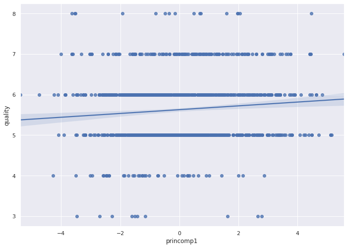
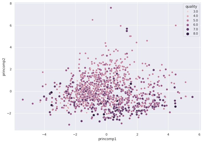
The graph of two principal components indicates poor predictive performance. We cannot draw a clean line that will predict the correct wine quality (depicted by the color and radius of the circles below).
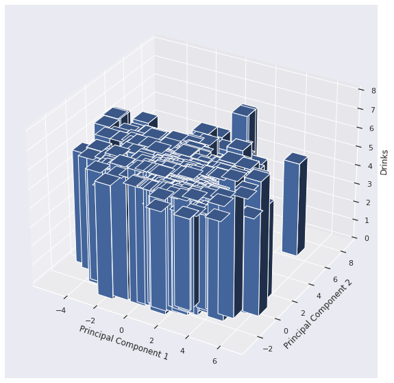
The 3D bar chart looks flat, which also indicates that we need more than two Principal Components.
How many Principal Components should we use? The eigenvalues record the variance for each eigenvector:
print(pca.explained_variance_)
[3.0807826  1.84947941 1.62211745 1.23466434 0.96610121 0.68122053
 0.58218232 0.40963393 0.3487236  0.17406732]
If we eyeball the vector of eigenvalues, we see that the first seven (7) or so principal components contain most of the variance.
When we reduce the dimensionality of the data set to seven, and apply the two algorithms, we witness the following results:
| Approach | Dims | RMSE |
|---|---|---|
| Linear Model | 7 | 0.633 |
| DNN | 7 | 0.645 |
| DNN | 11 | 0.648 |
| Linear Model | 11 | 0.706 |
| Linear Model | 2 | 0.735 |
| Guess Mean | N/A | 0.801 |
The dimensionality reduced Linear Model wins.
Can Google AutoML tables beat the dimensionality reduced Linear Model? Let's find out!
Import the UCI Wine Data Set
Download the Wine Data Set from UCI to your workstation and execute the following two actions.
- Replace all semi-colons (;) with commas (,)
- Replace all spaces with underscores (_)
See a snippet of wine.csv below:
fixed_acidity,volatile_acidity,citric_acid,residual_sugar,chlorides,free_sulfur_dioxide,total_sulfur_dioxide,density,pH,sulphates,alcohol,quality
7.4,0.7,0,1.9,0.076,11,34,0.9978,3.51,0.56,9.4,5
7.8,0.88,0,2.6,0.098,25,67,0.9968,3.2,0.68,9.8,5
7.8,0.76,0.04,2.3,0.092,15,54,0.997,3.26,0.65,9.8,5
11.2,0.28,0.56,1.9,0.075,17,60,0.998,3.16,0.58,9.8,6
7.4,0.7,0,1.9,0.076,11,34,0.9978,3.51,0.56,9.4,5
7.4,0.66,0,1.8,0.075,13,40,0.9978,3.51,0.56,9.4,5
7.3,0.65,0,1.2,0.065,15,21,0.9946,3.39,0.47,10,7

               <snip>

6.3,0.51,0.13,2.3,0.076,29,40,0.99574,3.42,0.75,11,6
5.9,0.645,0.12,2,0.075,32,44,0.99547,3.57,0.71,10.2,5
6,0.31,0.47,3.6,0.067,18,42,0.99549,3.39,0.66,11,6
Follow the process that we used to (attempt to) import the BUPA data set above. Create a new bucket and folder if desired.
I created a bucket named wine-quality-data and a folder named red.
After we click import Google will suggest that we close the window.
After about forty-five minutes, Google sends an email that reports a successful import.
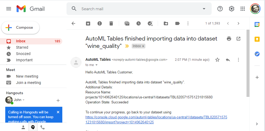
With our imported data set, we can now train the model.
Train the Model
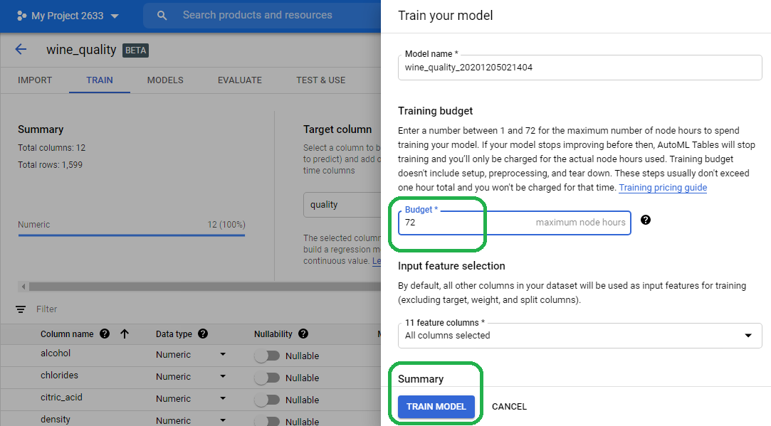
Click the Train tab in the console.
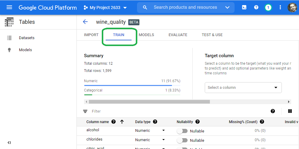
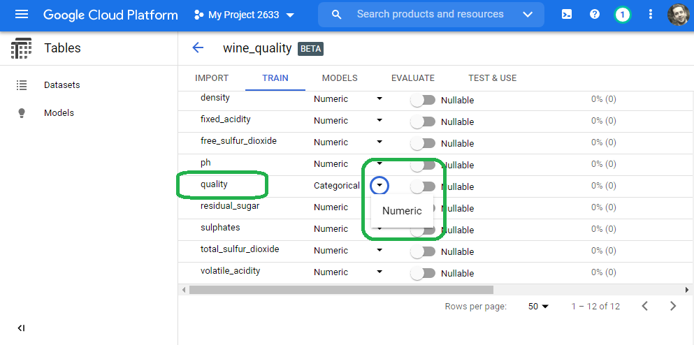
Scroll down to our target variable quality and change the data type from categorical to numeric.
Note: In the spirit of our earlier efforts, we select numeric to continue with the regression theme. If we want a classification model, then we can set data type to categorical
Scroll to the top and set the target variable to quality.
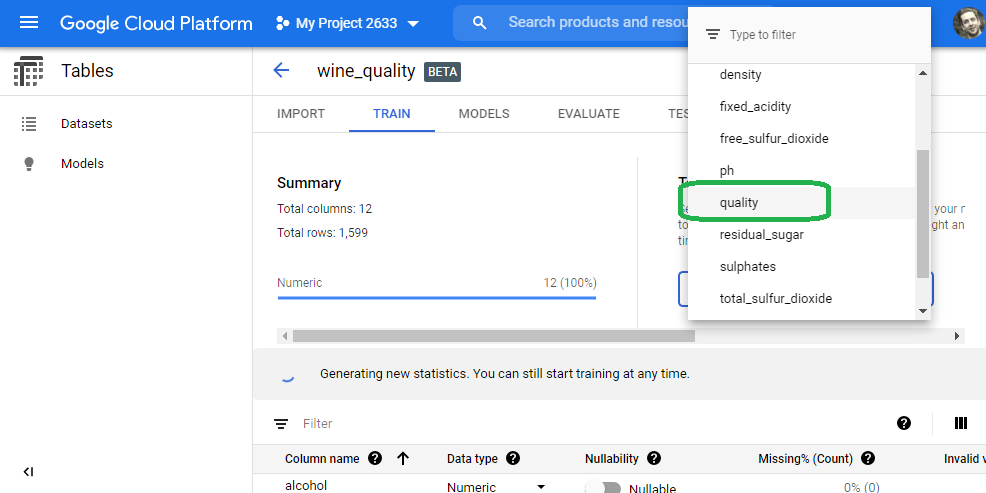
Select train model. We can limit the number of CPU hours (e.g. cost) if desired. I just set the value to the maximum. Our simple model will not consume these resources. Click Train Model.
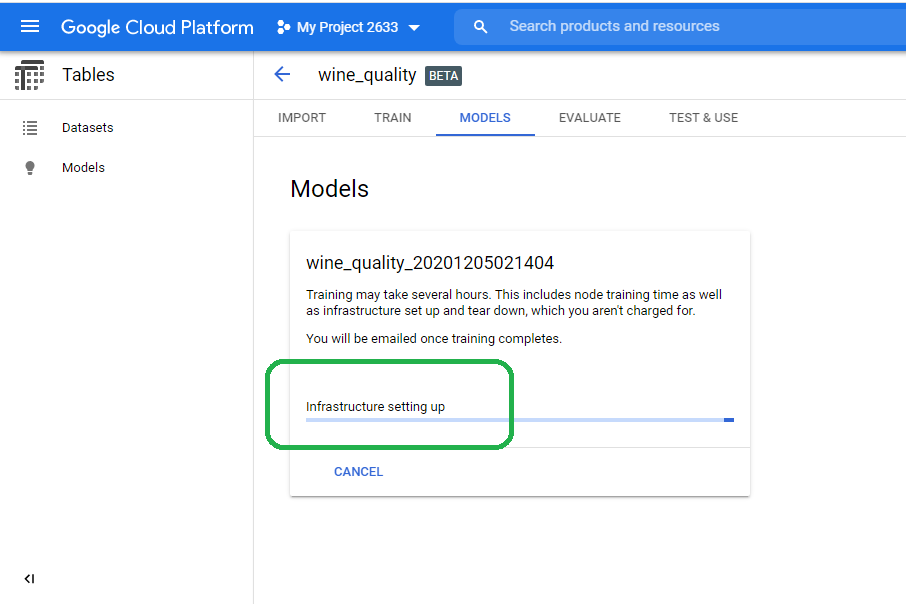
The Google singularity then gets to work and creates the infrastructure needed to train our model. We can close the browser. Google will email us a notification once they finish developing the model.
View Results
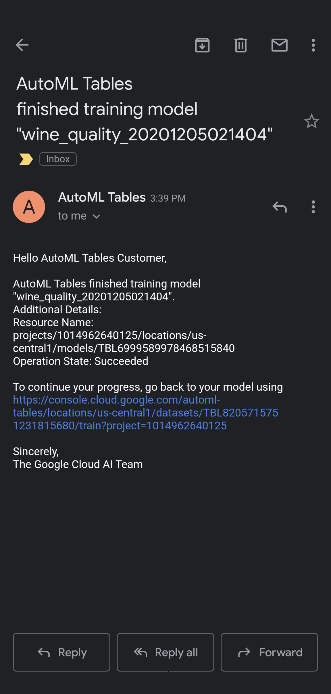
After a few hours, Google sends an email that notifies us of model completion.
Navigate back to the Tables service and click the Models tab. The GCP console presents the results.
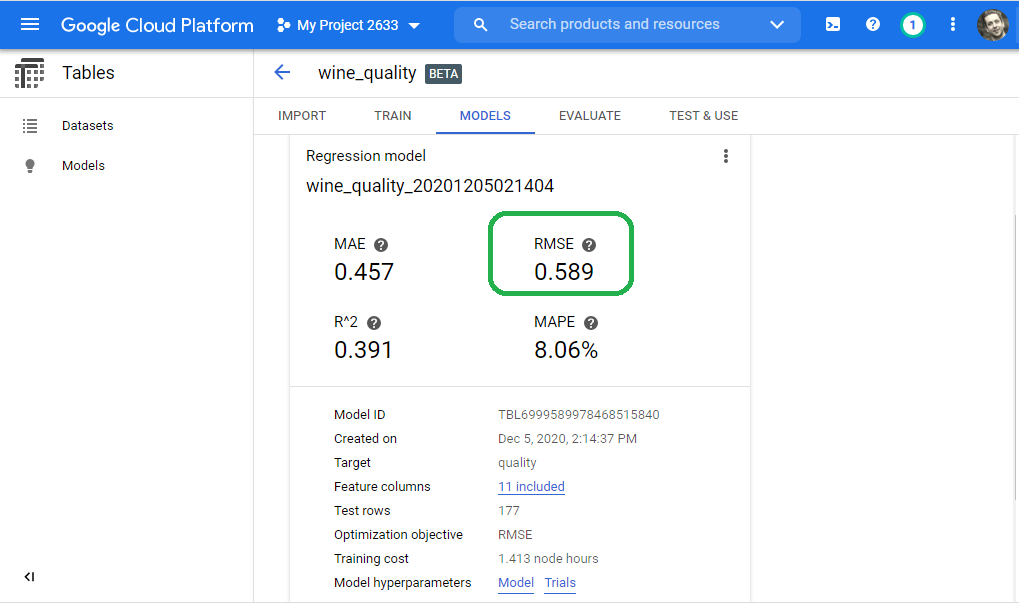
In summary, the Google AutoML Tables Beta service yields the best results:
| Approach | Dims | RMSE |
|---|---|---|
| AutoML Tables | 11 | 0.598 |
| Linear Model | 7 | 0.633 |
| DNN | 7 | 0.645 |
| DNN | 11 | 0.648 |
| Linear Model | 11 | 0.706 |
| Linear Model | 2 | 0.735 |
| Guess Mean | N/A | 0.801 |
NOTE: We achieved the best results with the least amount of work: Upload a CSV and click train!
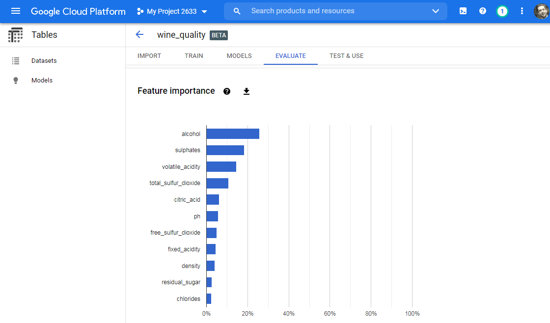
Model Meta Data
The service provides feature importance. Google reports that alcohol drives quality more than any other feature.
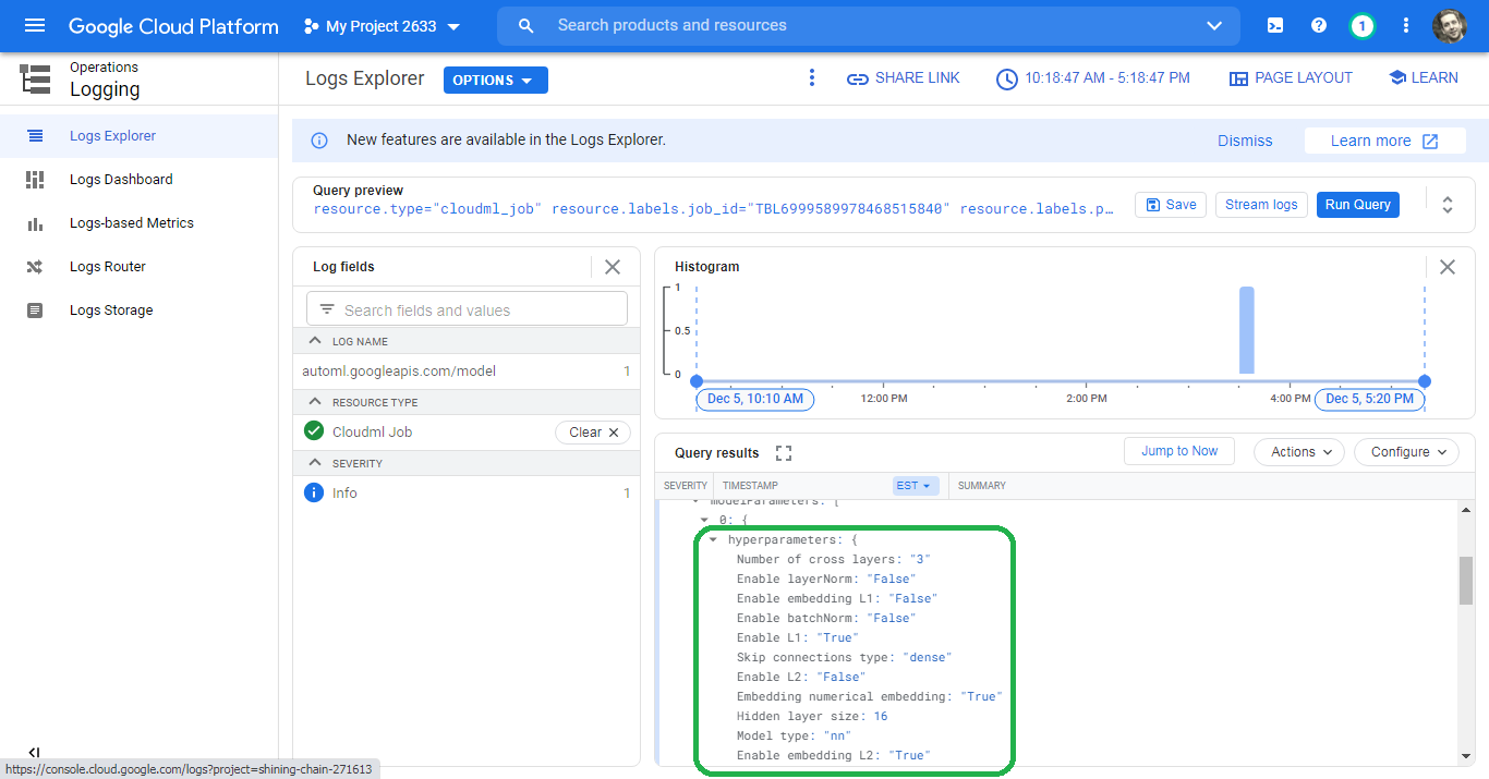
Model Hyperparameters under the Model tab re-directs us to the GCP Operations Logging console. These logs include the different scenarios for each iteration. Trial zero, for example, uses a Neural Network with sixteen (16) layers.
Trial fifteen uses a Gradient Boosted Decision Tree (GBDT).
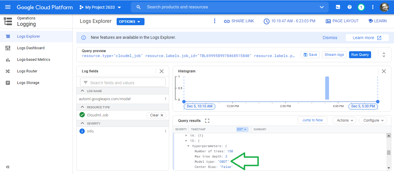
The logs provide a cumbersome UI to investigate the trials. Perhaps the Alpha service will clean up the UI and present a friendlier dashboard.
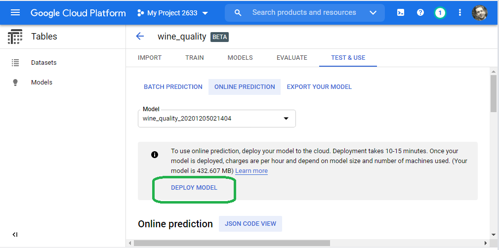
Deploy the Model
Now that we developed the model, we will deploy the model for use. The AutoML service provides one-click, no-code model deployment.
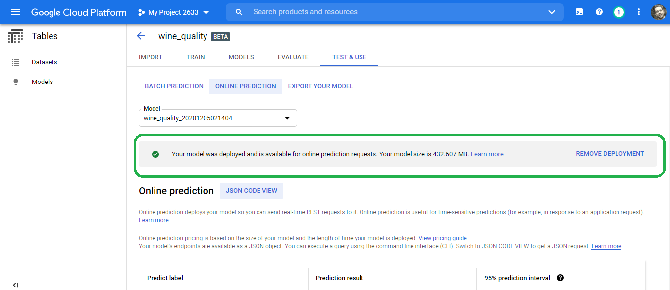
Click Test And Use --> Online Prediction --> Deploy Model.
Google once more deploys the model, and perhaps more importantly, the required infrastructure to enable model serving.
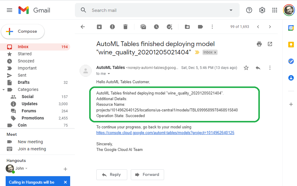
Google emails an alert once the model deployment completes.
Test the Model
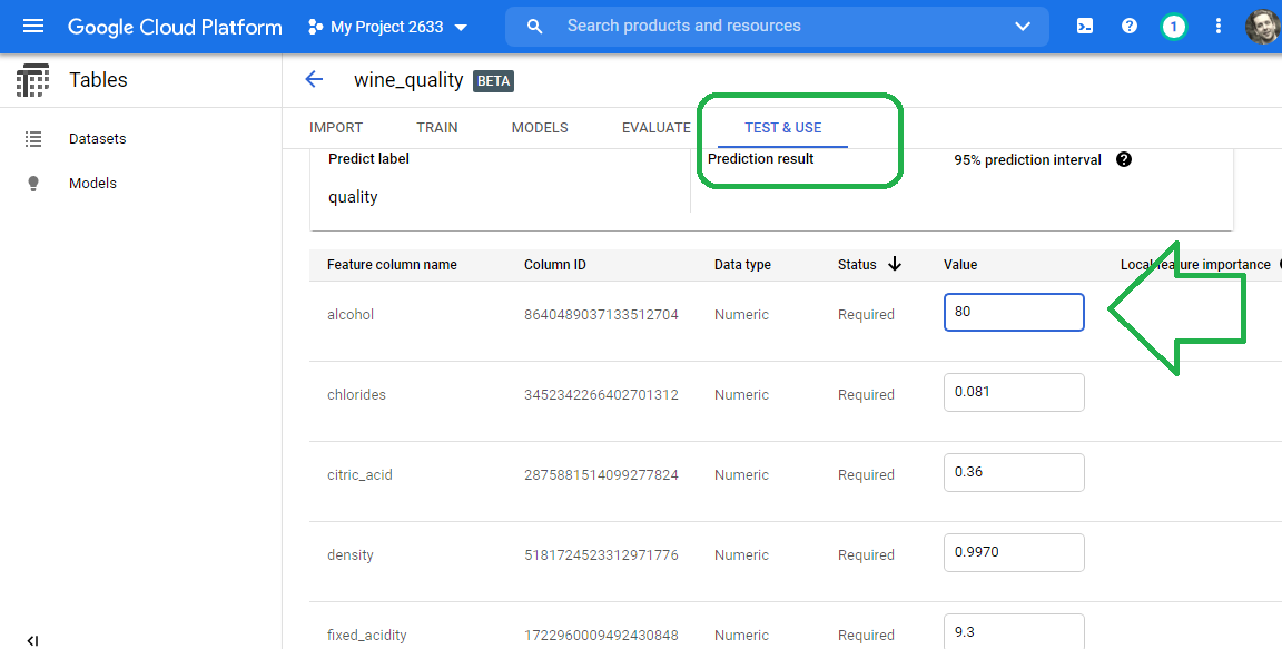
The online prediction tab provides a web form to test the model.
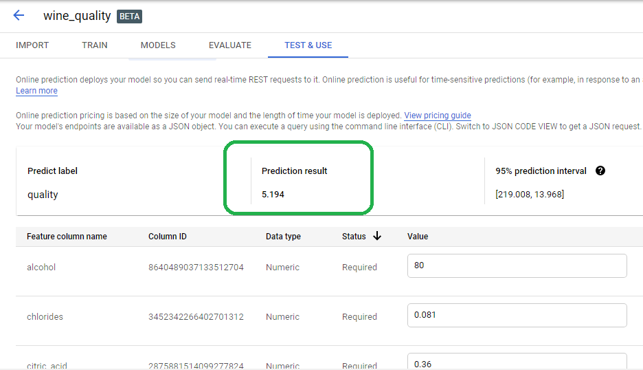
Scroll down to the alcohol field. What score can we expect for a 160 proof bottle of wine? Simply enter the number eighty into the alcohol field and then click test.
The model predicts our strong wine deserves a score of 5.194
The AutoML Tables Beta also service provides a REST API for machines to submit predictions to the model.
Billing
The AutoML Tables Beta service costs significantly less than our Vision model. We paid $28 for one and a half hour of compute time.
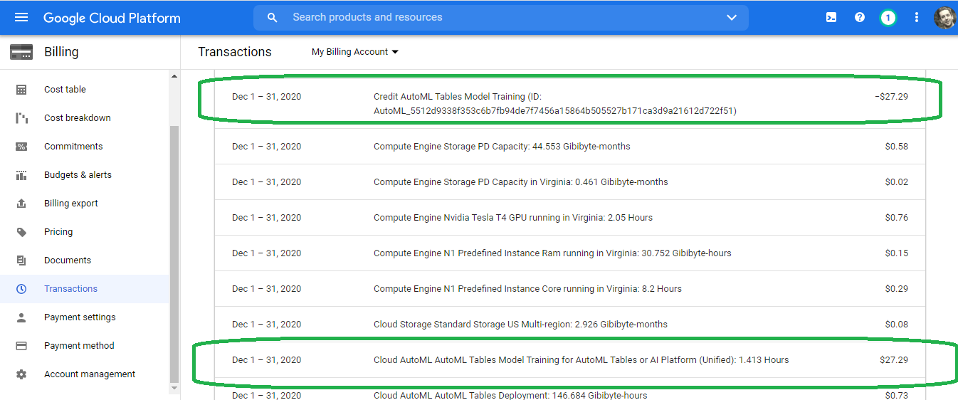
Google gave us a credit for the training, so we did not need to pay any out-of-pocket fee.
Conclusion
In this blog post we test-drove the Google AutoML Tables Beta service. The service did not accommodate our BUPA data, so we needed to pivot and try another Data Set, the UCI Wine Quality data set.
We used Pandas, SciKit Learn and TensorFlow 2.3 to wrangle, explore, normalize, visualize and split the Wine Quality data set. We used Keras 2.3 to train a linear model and DNN model and compared the results. We then iterated on dimensionality reduction approaches, converging on a good-enough number of features. PCA provided the vehicle to reduce dimensionality. The TensorFlow/ Keras/ Pandas approach required domain knowledge of AI/ML concepts and also required familiarity with various Python libraries and methods. In other words, the Python approach required considerable Math, Data Science and Software Development skills.
The Google AutoML Tables Beta service obviated the need for subject matter expertise. We simply uploaded a CSV and clicked run. Google took care of the rest. The AutoML Tables Beta service, therefore, democratizes the power of AI/ML and puts the technology in the hands of non-technical business users. I look forward to the Alpha release of this service.