I've previously discussed the Reduced Coloumb Energy Neural Net algorithm on this site. I wrote the algorithm in Matlab, which uses index based logic to select, filter, wrangle and process data. Today I will refactor the Matlab code to Tidyverse. Tidyverse uses forward pipe operators to flow data through the data processing steps.

The example RCE algorithm assigns a class to data based on whether or not the data points live inside "footprints" of training data. If a visual walk through the RCE algorithm interests you, take a minute to read my post titled A Graphical Introduction to Probabalistic Neural Networks.
The following graphic captures an animation of the RCE NN Algorithm in action.
You can find the original Matlab script and the new R script on GitHub.
Loading Data
The algorithm loads the BUPA liver disorders database from the University of California, Irvine (UCI) machine learning repository.
Matlab
In Matlab, we encode the CSV into a matrix with brackets and assignment.
data = [85,92,45,27,31,0.0,1
85,64,59,32,23,0.0,2
86,54,33,16,54,0.0,2
91,78,34,24,36,0.0,2
87,70,12,28,10,0.0,2

...

98,77,55,35,89,15.0,1
91,68,27,26,14,16.0,1
98,99,57,45,65,20.0,1];
Tidyverse
Tidyverse allows us to read the raw CSV and store it in a Tibble.
In addition to storing the CSV data in a Tibble, we use the readr library to add column names (col_names) and an ID column (rowid_to_column).
I discuss the definitions of the column names in the next section
library("readr")
library("dplyr")
library("magrittr")
library("purrr")
library("tidyr")

columns <- c( "mcv", "alkphos", "sgpt", "sgot", "gammagt", "drinks_num", "select")

Bupa.Tib <- read_csv( "bupa.data", col_names = columns ) %>%
  tibble::rowid_to_column("id")
Selecting Features
The BUPA data includes six features and two classes (one for alcohol related liver disorder, and one for alcohol unrelated liver disorder).
The six (6) BUPA features include:
- mean corpuscular volume (mcv)
- Four chemical markers
- alkaline phosphotase (alkphos)
- alamine aminotransferase (sgpt)
- aspartate aminotransferase (sgot)
- gamma-glutamyl transpeptidase (gammagt)
- half-pint equivalents of alcohol per day (drinks)
I discussed the salient features in my RCE writeup. Three features, "alkphos", "sgpt" and "gammagt" stand out in terms of the algorithm's classification performance. We still would like to provide the Data Scientist with flexibility in selecting the features, for "what if" scenarios, so we write our code to accommodate an arbitrary number of features.
Matlab
In Matlab, we use the column index to select the features. In this case, we use alkphos == 2, sgpt == 5, and gammagt == 6.
feats = [2 5 6];
Tidyverse
Tidyverse allows us to name the columns and then select by name.
When we created Bupa.Tib we named the columns, so now we can select columns by name.
We create a list that records the column names that we intend to keep.
features <- c( "alkphos", "sgpt", "gammagt")
Creating the training set
Matlab
In Matlab, we sort the data by the class, which the matrix stores in column seven (7).
We then use index operations to select all features, excluding the class.
Then we select the desired features using the feats array. A function, named prepare_uncoded wraps this operation.
function [data] = prepare_uncoded(data,feats)
    data = sortrows(data,7);
    data = data(:,1:6);
    data = data(:,feats);
end
We create two separate matrices, one that includes the first seventy-two (72) rows, and one that includes the bottom seventy-two (72) rows. Since we sorted by class in the function above, we produce one matrix of train patterns that contains class one, and one that contains train patterns of class two.
data = prepare_uncoded(data,feats);

class1 = data(73:144,:)';
class2 = data(145:216,:)';
Tidyverse
The MagrittR package of Tidyverse enables a pipe forward operator. The pipe forward operation provides a more readable feature selection operation.
We use filter to filter points of each class, select to select the features and slice to pull specific rows.
NOTE: Just to disambiguate, Irvine named the class column select, so we filter based on the value of the select column.
class_1_training_patterns <- c( 73:144 )
class_2_training_patterns <- c( 1:72 )

Class.1.Train.Tib <- Bupa.Tib %>%
  filter( select == 1 ) %>%
  select( id, features) %>%
  slice( class_1_training_patterns )

Class.2.Train.Tib <- Bupa.Tib %>%
  filter( select == 2 ) %>%
  select( id, features) %>%
  slice( class_2_training_patterns )
Find Radii
The RCE NN algorithm requires us to find the radii between a train point and the nearest train point of the opposite class.
We compute the euclidean distance to all other training points of the other class, and store the distance (named lambda) of the closest one.
Matlab
In Matlab, we create a function that ingests both the Class 1 and Class 2 training matrices, along with epsilon and lambda max. Lambda max provides an upper bound in terms of the maximum radius the algorithm will consider. Epsilon provides a very small value that we subtract from the calculated lambda. For more details, see my writeup of the RCE NN algorithm.
The Matlab code performs Matrix operations via nested functions to calculate the euclidean distance to all other points and then record the minimum.
In addition, the code uses a for loop to iterate through every training pattern.
The function iterates through each training point, calculates the distance to every other training point (stored in the two Class matrices) and keeps the minimum.
It then returns two arrays that contain lambda, one array per class.
function [lambda_1, lambda_2] = rce_train(class1,class2,eps,lambda_max)
 %Find number of train patterns (colums)
    n_c1p = size(class1,2);
    n_c2p = size(class2,2);

    for i=1:n_c1p
            x_hat = min(sqrt(sum((class2-class1(:,i)*ones(1,n_c1p)).^2)));
            lambda_1(i) = min(x_hat - eps, lambda_max);
    end
    for i=1:n_c2p
            x_hat = min(sqrt(sum((class1-class2(:,i)*ones(1,n_c2p)).^2)));
            lambda_2(i) = min(x_hat - eps, lambda_max);
    end
end
We apply the function to the training matrices:
[lambda_1 lambda_2] = rce_train(class1,class2,eps,lambda_max);
Tidyverse
R best practices do not encourage for loops, since R follows a functional programming convention.
In addition, the MagrittR pipes allow us to avoid nested functions.
We first create a function find_lambda. I decided to process the data one class at a time, so this function only calculates the distance to training points of the other class, and not all data points as in the Matlab function above.
The find_lambda function takes a single observation (row of data) for a particular class, along with the entire Tibble that contains all data points of the other class. The function also ingests epsilon, lambda max and the features vector.
Not to overload terms too much, but the function includes a lambda function that calculates the Euclidean distance between two vectors.
The lambda function takes two vectors, the observation vector and a row from the other class Tibble, which I call x.
function(x) sqrt( sum( ( x - observation )^2 )
The Lambda function can perform calculations on vectors of any length, which provides Data Scientists flexiblity in choosing which features to include.
The find_lambda function follows, and I will explain it quickly line by line.
find_lambda <- function( observation, Other.Class.Tib, lambda_max, epsilon, features ) {
  Other.Class.Tib %>%
    select( features ) %>%
    mutate( euclid_dist = apply( . , 1, function(x) sqrt( sum( ( x - observation )^2 ) ) ) ) %>%
    select( euclid_dist ) %>%
    min() %>%
    min( . - epsilon, lambda_max ) }
We start with the Tibble that contains all observations of the other class, stored in Other.Class.Tib.
The function pipes the Tibble in its entirety to a select statement that selects all of the desired features.
We then use the mutate operator to create a new column named euclid_dist. This column stores the euclid_dist from the current observation (single vector) to every data point (row) in the Other.Class.Tib.
The apply operator tells Tidyverse to apply the Euclidean distance lambda function to every row in Other.Class.Tib and store the result for each row in the euclid_dist column.
Since we must accommodate vectors of arbitrary length we tell apply to input row wise data via the 1 in the second parameter in the function signature.
Once the apply operation completes, we have a column that records the distance to each data point in the Other.Class.Tib. We are only interested in the nearest data point of the other class so we select the euclid_dist column and find the min(). We then ensure that the minimum distance has length less than lambda max.
In summary, we supply the function with a single observation for a class, along with a Tibble that includes all observations for the other class. The function then returns a single value, the distance between the current observation and the nearest data point of the other class.
We are not done yet. We must apply this function to every training point in the Class under observation.
# Find Lambda for Class 1 Training patterns
Class.1.Train.Tib %<>%
  select( features ) %>%
  mutate( lambda = apply(. , 1, function(x) find_lambda(x,
                                                        Class.2.Train.Tib,
                                                        lambda_max,
                                                        epsilon,
                                                        features ) ) ) %>%
  mutate( id = Class.1.Train.Tib$id )

# Find Lambda for Class 2 Training patterns
Class.2.Train.Tib %<>%
  select( features ) %>%
  mutate( lambda = apply(. , 1, function(x) find_lambda(x,
                                                        Class.1.Train.Tib,
                                                        lambda_max,
                                                        epsilon,
                                                        features ) ) ) %>%
  mutate( id = Class.2.Train.Tib$id )
We pipe the entire Class.1.Train.Tib to a select function and then use the apply operation to execute find_lambda on every row of Class.1.Train tib. Although each iteration (application) of find_lambda inputs the entire Tibble of Class.2.Train.Tin, it returns a single value for lambda.
NOTE: The MagrittR %<>% operation pipes data forward and stores the final result of all chained operations back into initial variable
The following output tibble depicts what Class.1.Train.Tib looks like after application of find_lambda.
> Class.1.Train.Tib
# A tibble: 72 x 5
   alkphos  sgpt gammagt lambda    id
     <dbl> <dbl>   <dbl>  <dbl> <int>
 1      67    77     114  29.1    175
 2      71    29      52  10.5    176
 3      93    22     123  19.4    182
 4      77    86      31  26.8    183
 5      77    39     108  20.4    189
 6      83    81     201  58.3    190
 7      75    25      14   3.16   191
 8      56    23      12   6.48   192
 9      91    27      15   7.87   194
10      62    17       5   5.00   195
# ... with 62 more rows
The closest data point in Class 2, for example, to the first Class 1 observation exists 29.1 units away.
Classify the Data
We first take the remaining BUPA data to create test patterns for each class.
Matlab
In Matlab:
test_class1 = data(1:72,:)';
test_class2 = data(217:288,:)';
Tidyverse
In Tidyverse I decided to create one Tibble for all Test Patterns, via the bind_rows operation.
Test.Patterns <- Bupa.Tib %>%
  filter( select == 1 ) %>%
  slice( class_1_test_patterns ) %>%
  bind_rows( Bupa.Tib %>%
                filter( select == 2 ) %>%
                slice( class_2_test_patterns ) )
Once we have test data, we need to classify it.
Matlab
In Matlab, I wrote a function named rce_clasify. The function contains a ton of nested functions and a for loop.
Each training pattern includes a circular "footprint" around it that extends to the nearest point of the other class, with radius equal to the lambda we calculated above.
The rce_clasify function finds which footprint each test observation lies in.
function [cl] = rce_classify(class1,lambda_1,class2,lambda_2,test_patterns)
        %Test Patterns in form: num_features x num_patterns
        ind1 = []; ind2 = [];
        %Find number of train patterns (colums)
        n_c1p = size(class1,2);
        n_c2p = size(class2,2);
        num_test_patterns = size(test_patterns,2);
        for i = 1:num_test_patterns
            test_x = test_patterns(:,i);
            dist1 = test_x*ones(1,n_c1p)-class1;
            dist1 = sqrt(diag(dist1'*dist1))';

            dist2 = test_x*ones(1,n_c2p)-class2;
            dist2 = sqrt(diag(dist2'*dist2))';

            ind1 = find(dist1 < lambda_1);
            ind2 = find(dist2 < lambda_2);
            p = 3;
            if ~isempty(ind1)
                p = 1;
            end
            if ~isempty(ind2)
                p = 2;
            end
            if (~isempty(ind1) && ~isempty(ind2))
                p = 3;
            end
            cl(i) = p;
        end
end
Tidyverse
In the Tidyverse classification approach, we use nested functions in the logical sense, since our code exclusively uses pipes.
We create a generic function to discover how many "footprints" the given observation lives in.
Similar to the Matlab code above, we calculate the distance between an observation of the Test data and all of the training samples of a given class.
We then use the lambda values of the training samples to identify the count (nrow) of footprints the test data lives in.
rce_classify <- function( observation, Data.Tib, features ) {
  Data.Tib %>%
    select( features ) %>%
    mutate( euclid_dist = apply( . , 1, function(x) sqrt( sum( ( x - observation )^2 ) ) ) ) %>%
    filter( euclid_dist < Data.Tib$lambda ) %>%
    nrow
}
Without getting too complicated, we pass the Test data to a function that uses rce_classify to detect the number of hits against each class of Training data. First it finds the hits against Class.2.Training.Tib, and then it finds the hits against Class.1.Training.Tib.
The new function rce_classify_tib then uses the number of hits for each class to classify the data. In this example, we use a voting approach, although you can tailor the algorithm to classify a test point as ambiguous if it hits either zero or more than one class.
rce_classify_tib <- function(Test.Data.Tib, Class.One.Train.Tib, Class.Two.Train.Tib, features) { Test.Data.Tib %<>%
  select( features ) %>%
  mutate( class.2.hits = apply( . , 1, function(x) rce_classify( x, Class.Two.Train.Tib , features ) ) ) %>%
    mutate( id = Test.Data.Tib$id )

Test.Data.Tib %<>%
  select(features) %>%
  mutate( class.1.hits = apply( . , 1, function(x) rce_classify( x, Class.One.Train.Tib, features ) ) ) %>%
  mutate( class.2.hits = Test.Data.Tib$class.2.hits,
          id = Test.Data.Tib$id ) %>%
  mutate( rce_class = ifelse( test = class.1.hits > class.2.hits,
                              yes = 1,
                              no = ifelse( test = class.2.hits > class.1.hits,
                                           yes = 2,
                                           no = 3)))
  return(Test.Data.Tib)
}
We then apply these functions to our data.
Matlab
In Matlab:
    cl1 = rce_classify(class1,lambda_1,class2,lambda_2,test_class1);
    cl2 = rce_classify(class1,lambda_1,class2,lambda_2,test_class2);
Tidyverse
In Tidyverse:
Test.Patterns %<>%
  rce_classify_tib(Class.1.Train.Tib, Class.2.Train.Tib, features)
Graphing RCE NN
We can graph the RCE NN in action by creating a uniform data grid and running rce_classify against every point.
First, create the data grid. We find the highest valued observation in the data set, in order to ensure that our graph includes this data point.
max_obs <- Class.1.Train.Tib %>%
  bind_rows(Class.2.Train.Tib) %>%
  select(features) %>%
  max

test_grid <- expand.grid( seq( 0, max_obs * 1.1, length.out = 50 ),
                          seq( 0, max_obs * 1.1, length.out = 50 ),
                          seq( 0, max_obs * 1.1, length.out = 50 ) )
names( test_grid ) <- features
Now we apply the classification to every test data point, in order to blanket the entire canvas.
Note: This will take a long time. If you don't want to wait, you can execute: test_grid = readxl::read_xlsx("NinetyK.xlsx")
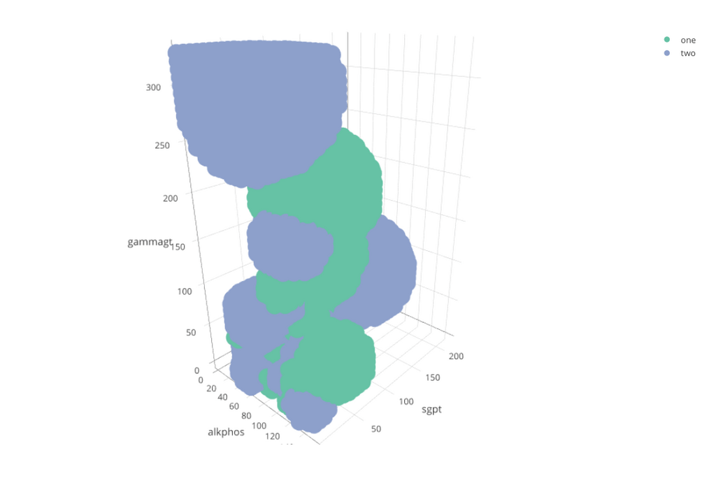
You can then use Plotly to generate a Three Dimensional image that you can rotate.
library("plotly")
test_grid %>% filter( rce_class != 3 ) %>%
  mutate( rce_class = ifelse( test = rce_class == 1,
                              yes  = "one",
                              no  = "two") ) %>%
  plot_ly( x = ~alkphos, y = ~sgpt, z = ~gammagt , color = ~rce_class )
If you would like to see a 2D graph, then re-run the script using two features.
features <- c( "alkphos", "sgpt")
Create a test grid using two dimensions and classify.
test_grid <- expand.grid( seq( 0, max_obs * 1.1, length.out = 300 ), seq( 0, max_obs * 1.1, length.out = 300 ) )
names( test_grid ) <- features

test_grid %<>%
  as_tibble %>%
  tibble::rowid_to_column("id") %>%
  rce_classify_tib( Class.1.Train.Tib, Class.2.Train.Tib, features)
You can just load the pre-processed data instead of waiting.
test_grid = readxl::read_xlsx("NinetyK.xlsx")
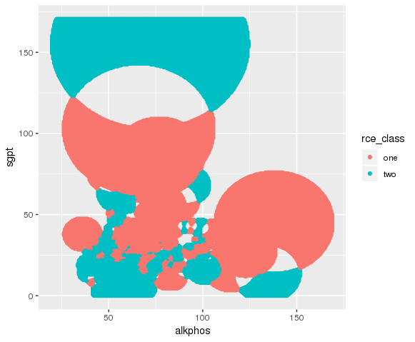
Here I plot using Grammer of Graphics.
ggplot( ) +
  geom_point( data = test_grid %>% filter( rce_class == 1 ), aes(x = alkphos, y = sgpt, color = class.1.hits )) +
  geom_point( data = test_grid %>% filter( rce_class == 2 ), aes(x = alkphos, y = sgpt, color = class.2.hits ))
Conclusion
This blog post described how to convert a Matlab script that uses for loops and nested function into a functional, pipe based Tidyverse script.
If you enjoyed this, you may enjoy these other Machine Learning posts.
- A New Exemplar Machine Learning Algorithm (Part 1: Develop)
- A New Exemplar Machine Learning Algorithm (Part 2: Optimize)
- Applying a Reduced Coulomb Energy (RCE) Neural Network Classifier to the Bupa Liver Disorders Data Set
- A Graphical Introduction to Probabilistic Neural Networks - Normalization and Implementation