In part one of this two-part series, I developed a Reduced Columb Energy (RCE) classifier in Python. RCE calculates hit footprints around training data and uses the footprints to classify test data.
RCE draws a circle around each labeled training observation, with a radius (lambda) that stops at the closest labeled training point in the opposite class. Each circle indicates the hit footprint for that class.
In part one I ran RCE for one epoch on a two-feature training set to achieve an F1 Score of 0.42 and ambiguity of 26.6%.
In this blog post, I will introduce and tune hyperparameters to improve model success and reduce ambiguity. I will investigate the number of principal components and tune r.
r indicates the maximum value for Lambda and puts an upper limit on the maximum size of each circle that represents a given hit footprint.
I will also see how RCE performs with a reduced training set. In Pattern Classification Using Neural Networks (IEEE Communications Magazine, Nov. 1989) Richard P. Lippman writes:
This classifier is similar to a k-nearest neighbor classifier in that it adapts rapidly over time, but it typically requires many fewer exemplar nodes than a nearest neighbor classifier.
Tune Number of Features
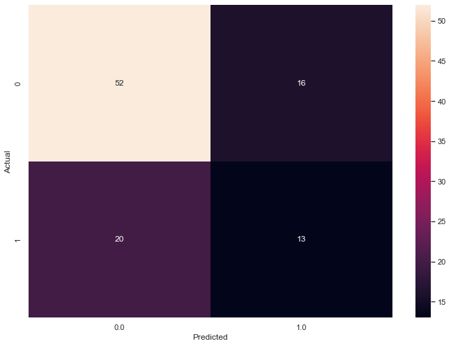
Last time, I left off with the following confusion matrix for the two principal component scenario. In that scenario, I applied RCE to the diabetes dataset after I used Principal Component Analysis (PCA) to reduce the data set down to two features.
Our RCE algorithm trained a model with an F1 Score of 0.42 and ambiguity of 26.6%.
calc_success(test_df)
{'f1_score': 0.42424242424242425,
 'ambiguity': 0.2662337662337662}
Three Principal Components
I use the following code to reduce the diabetes training dataset down to three components and yield a Pandas dataframe named test_df.
pca_train = PCA(n_components=3)
pca_train.fit(normalizer(train_features))

train_df = pd.DataFrame(pca_train.transform(normalizer(train_features)),
                                     columns = ['princomp1',
                                                'princomp2',
                                                'princomp3'],
                                     index=train_features.index).assign(outcome = train_labels)
train_df['lambda'] = train_df.apply(lambda X: find_lambda(train_df, X),axis = 1)

pca = PCA(n_components=3)
pca.fit(normalizer(test_features))
test_df = pd.DataFrame(pca.transform(normalizer(test_features)),
                                     columns = ['princomp1',
                                                'princomp2',
                                                'princomp3'],
                                     index=test_features.index)
I then call my classify_data() function to classify the data.
test_df = classify_data(train_df, test_df)
I attach the labels to the classified data frame for the confusion matrix.
test_df = test_df.assign(actual=test_labels)
confusion_matrix = pd.crosstab(test_df['actual'], test_df['classification'], rownames=['Actual'], colnames=['Predicted'])

sns.heatmap(confusion_matrix, annot=True)
plt.show()
Three features yield the following confusion_matrix:
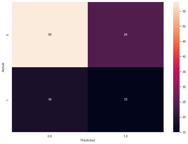
My calc_success() function returns f1_score and ambiguity.
from sklearn.metrics import f1_score

def calc_success(test_df):
    unambiguous_df = test_df.dropna()
    ambiguity = (test_df.shape[0] - unambiguous_df.shape[0])/test_df.shape[0]
    f1 = f1_score(unambiguous_df.actual, unambiguous_df.classification)
    return { "f1_score" : f1, "ambiguity" : ambiguity}

calc_success(test_df)
Both F1 (bad) and ambiguity (good) decrease with an extra principal component.
{'f1_score': 0.41666666666666663,
'ambiguity': 0.2532467532467532}
Four Principal Components
The following code fits the train dataset to four principal components, classifies the resulting data frame and then plots the confusion matrix.
pca = PCA(n_components=4)
pca.fit(normalizer(train_features))
pca_train_features_df = pd.DataFrame(pca.transform(normalizer(train_features)),
                                     columns = ['princomp1',
                                                'princomp2',
                                                'princomp3',
                                                'princomp4'],
                                     index=train_features.index)
train_df = pca_train_features_df.assign(outcome = train_labels)
train_df['lambda'] = train_df.apply(lambda X: find_lambda(train_df, X),axis = 1)


pca = PCA(n_components=4)
pca.fit(normalizer(test_features))
test_df = pd.DataFrame(pca.transform(normalizer(test_features)),
                                     columns = ['princomp1',
                                                'princomp2',
                                                'princomp3',
                                                'princomp4'],
                                     index=test_features.index)

test_df = classify_data(train_df, test_df)
test_df = test_df.assign(actual=test_labels)
confusion_matrix = pd.crosstab(test_df['actual'],test_df['classification'], rownames=['Actual'], colnames=['Predicted'])

sns.heatmap(confusion_matrix, annot=True)
plt.show()
The F1 score increases slightly and the ambiguity shoots up.
{'f1_score': 0.41935483870967744,
 'ambiguity': 0.34415584415584416}
Five Principal Components
I use the following code to look at the five Principal Component scenario.
pca = PCA(n_components=5)
pca.fit(normalizer(train_features))
pca_train_features_df = pd.DataFrame(pca.transform(normalizer(train_features)),
                                     columns = ['princomp1',
                                                'princomp2',
                                                'princomp3',
                                                'princomp4',
                                                'princomp5'],
                                     index=train_features.index)
train_df = pca_train_features_df.assign(outcome = train_labels)
train_df['lambda'] = train_df.apply(lambda X: find_lambda(train_df, X),axis = 1)


pca = PCA(n_components=5)
pca.fit(normalizer(test_features))
test_df = pd.DataFrame(pca.transform(normalizer(test_features)),
                                     columns = ['princomp1',
                                                'princomp2',
                                                'princomp3',
                                                'princomp4',
                                                'princomp5'],
                                     index=test_features.index)

test_df = classify_data(train_df, test_df)
test_df = test_df.assign(actual=test_labels)
confusion_matrix = pd.crosstab(test_df['actual'], test_df['classification'], rownames=['Actual'], colnames=['Predicted'])

sns.heatmap(confusion_matrix, annot=True)
plt.show()

Five principal components decrease the F1 score and increase the ambiguity.
{'f1_score': 0.3928571428571428,
'ambiguity': 0.36363636363636365}
Principal Component Results
The following table captures the results of the investigation.
| P | f1 | Ambig. |
|---|---|---|
| 2 | .424 | .266 |
| 3 | .417 | .253 |
| 4 | .419 | .344 |
| 5 | .393 | .363 |
Tune the Radius
The original find_lambda formula increases the radius of the hit footprint until the footprint collides with a point of the opposite class.
def find_lambda(df, v):
  return ( np
            .linalg
            .norm(df
                    .loc[df['outcome'] != v[-1]]
                    .iloc[:,:-1]
                    .sub(np
                           .array(v[:-1])),
                  axis = 1)
            .min())
In part one, we see the footprints that result from unbounded radii.
I can add the following conditional to scope the footprint to a set maximum radius, r.
def find_lambda(df, v, r):
    lambda_var = ( np
                     .linalg
                     .norm(df
                             .loc[df['outcome'] != v[-1]]
                             .iloc[:,:-1]
                             .sub(np
                                    .array(v[:-1])),
                           axis = 1)
                     .min())
    return r if lambda_var > r else lambda_var
I add r to the find_lambda function. (Note the vocabulary overload, the following code uses a lambda function named find_lambda).
train_df['lambda'] = train_df.apply(lambda X: find_lambda(train_df,
                                                          X,
                                                          0.1),
                                                          axis = 1)
A scoped radius of maximum 0.1 creates the following footprints.
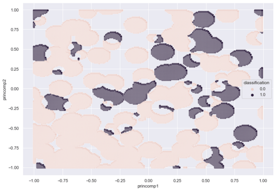
The following code creates, labels and plots a three dimensional dataset, with r set to 3.
# Generate 3 Principal Components for training
pca = PCA(n_components=3)
pca.fit(normalizer(train_features))
pca_train_features_df = pd.DataFrame(pca.transform(normalizer(train_features)),
columns = ['princomp1',
'princomp2',
'princomp3'],
index=train_features.index)
# Re-attach the labels for training
train_df = pca_train_features_df.assign(outcome = train_labels)
# ID Lambda for each datum
train_df['lambda'] = train_df.apply(lambda X: find_lambda(train_df, X, 3),axis = 1)
# Generate a 3D grid for data viz
class_3d_df = pd.DataFrame([(x,y,z) for x in range(-25,25) for y in range(-25,25) for z in range(-25,25)],
columns = ['princomp1',
'princomp2',
'princomp3'])/25
# Classify each point of the grid for data viz
class_3d_df = classify_data(train_df, class_3d_df)
plot_3d(class_3d_df,
'classification',
'princomp1',
'princomp2',
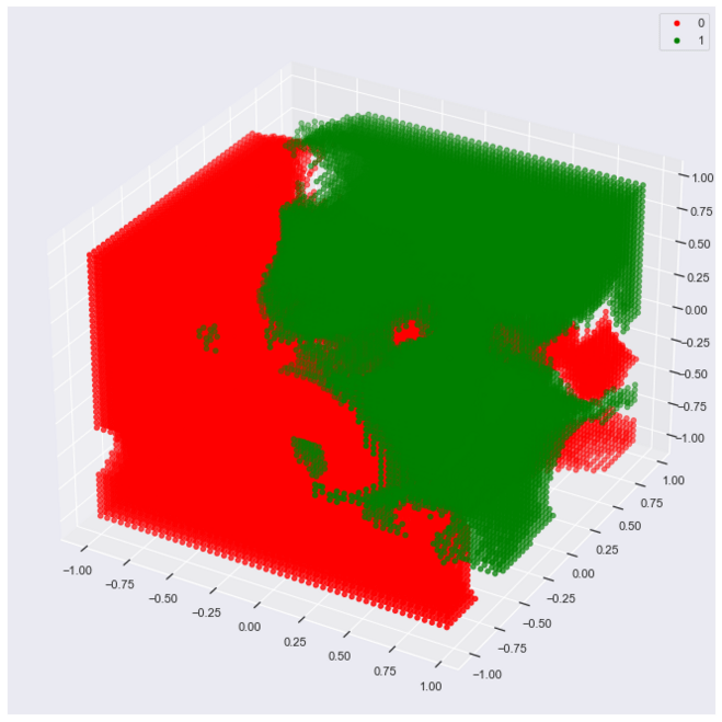
'princomp3')
This plot captures the hit footprints in 3d, with each footprint a sphere versus a circle (2d case).
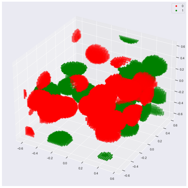
Re-run the code above with the following edit to set r to 0.15:
train_df['lambda'] = train_df.apply(lambda X: find_lambda(train_df,
                                                          X,
                                                          0.15),
                                                          axis = 1)
With a smaller r we get a better view of the spheres that show the hit footprints.
r provides a hyperparameter to the RCE algorithm. Different values of r will produce different results in terms of model effectiveness.
I create a function named hyperparameter_tune that applies RCE to a fresh train dataset, constrained by a given value for r and returns the f1 score and ambiguity.
def hyperparameter_tune(radius):
    train_df = raw_train_df.copy()
    train_df['lambda'] = train_df.apply(lambda X: find_lambda(train_df, X, radius),axis = 1)

    test_df = raw_test_df.copy()
    test_df = classify_data(train_df,test_df)
    test_df = test_df.assign(actual=test_labels)
    return calc_success(test_df)
I then iterate through one-hundred epochs, changing the values for r, spread between zero and one.
loss = []

for x in range(0,100):
    if x == 0:
        pass
    else:
        score = hyperparameter_tune(x/100)
        score['r'] = x/100
        loss.append(score)
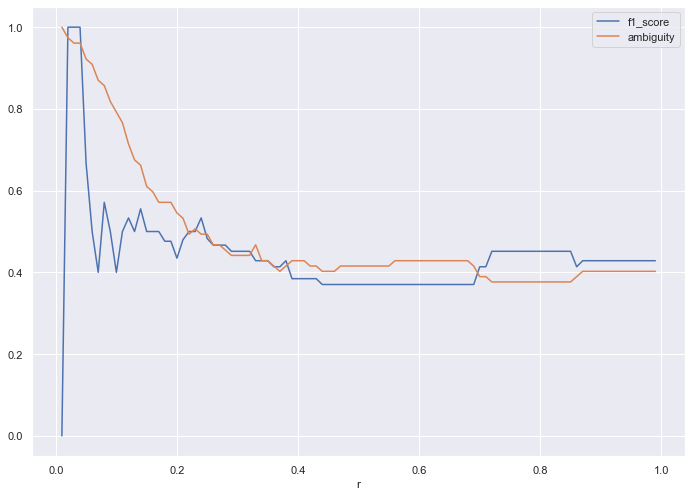
I then plot the results, to identify the optimal r value for the given train dataset.
pd.DataFrame(loss).set_index('r').plot()
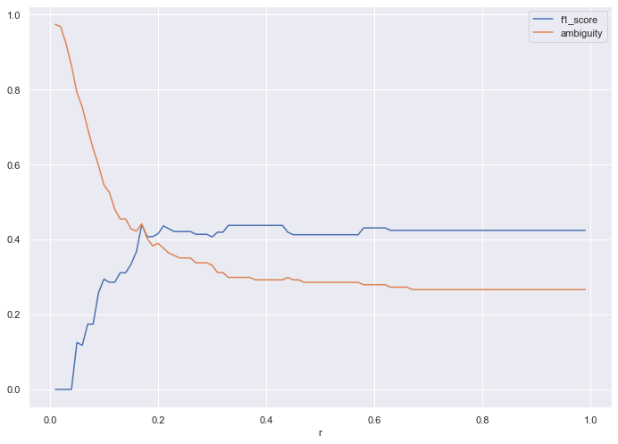
r = 0.58 yields the ideal results, with an f1_score of 0.43 and ambiguity of 0.27.
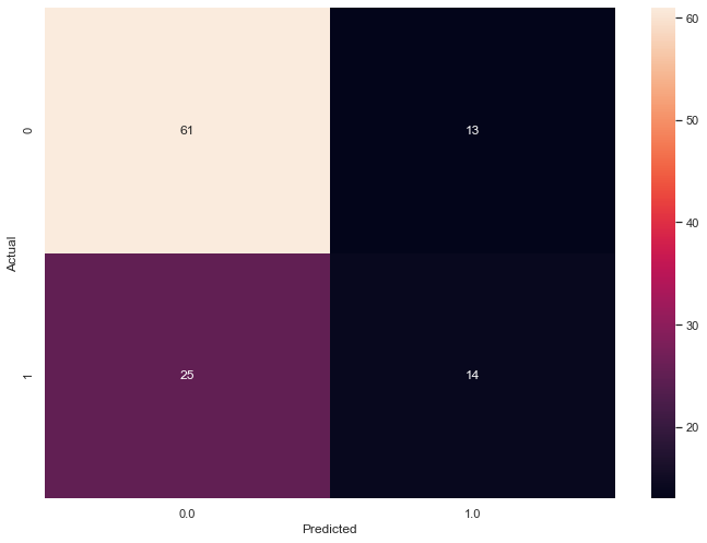
The following confusion matrix captures the results for r=0.58.
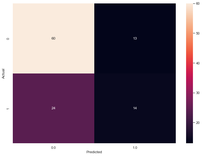
Tune the Algorithm
Our Algorithm declares regions with either (1) no footprint, or (2) overlapping footprints ambiguous. The Python code follows:
# Original
def classify_data(training_df, class_df):
    # find the hits
    class0_hits = class_df.apply(lambda X: find_hits(training_df, X, 0),axis = 1)
    class1_hits = class_df.apply(lambda X: find_hits(training_df, X, 1),axis = 1)
    # add the columns
    class_df = class_df.assign( class0_hits = class0_hits)
    class_df = class_df.assign( class1_hits = class1_hits)
    # ID ambiguous, class 0 and class 1 data
    class_df['classification'] = np.nan
    class_df['classification'] = class_df.apply(lambda X: 0 if X.class0_hits > 0 and X.class1_hits == 0 else X.classification, axis = 1)
    class_df['classification'] = class_df.apply(lambda X: 1 if X.class1_hits > 0 and X.class0_hits == 0 else X.classification, axis = 1)
    return class_df
To decrease ambiguity, I add vote logic to the code. In this case, overlapping regions will have a winner class in the case where one class includes more exemplars than the other.
# Reduce Ambiguity
def classify_data(training_df, class_df):
    # find the hits
    class0_hits = class_df.apply(lambda X: find_hits(training_df, X, 0),axis = 1)
    class1_hits = class_df.apply(lambda X: find_hits(training_df, X, 1),axis = 1)
    # add the columns
    class_df = class_df.assign( class0_hits = class0_hits)
    class_df = class_df.assign( class1_hits = class1_hits)
    # ID ambiguous, class 0 and class 1 data
    class_df['classification'] = np.nan
    class_df['classification'] = class_df.apply(lambda X: 0 if X.class0_hits > X.class1_hits else X.classification, axis = 1)
    class_df['classification'] = class_df.apply(lambda X: 1 if X.class1_hits > X.class0_hits else X.classification, axis = 1)
    return class_df
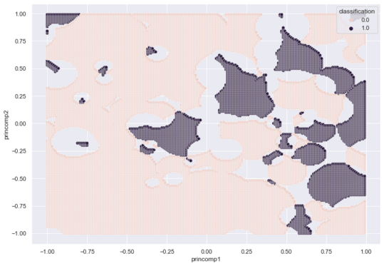
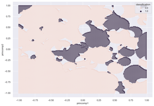
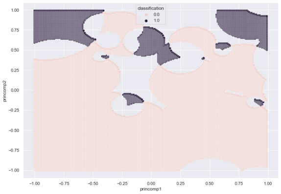
The Voting RCE algorithm produces a 2d footprint map with a high concentration of Class Zero regions.
I tune r for the new algorithm and plot the results using the same code above.
loss = []

for x in range(0,100):
    if x == 0:
        pass
    else:
        score = hyperparameter_tune(x/100)
        score['r'] = x/100
        loss.append(score)

pd.DataFrame(loss).set_index('r').plot()
The tuning identifies an ideal r of 0.40, which yields an f1_score of 0.4 and ambiguity of 0.2. The ambiguity drops from the non-voting algorithm, which yielded .27.
Small Training Sets
In Pattern Classification Using Neural Networks (IEEE Communications Magazine, Nov. 1989) Richard P. Lippman writes that RCE handles small training sets with aplomb:
This classifier is similar to a k-nearest neighbor classifier in that it adapts rapidly over time, but it typically requires many fewer exemplar nodes than a nearest neighbor classifier.
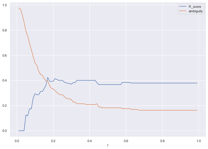
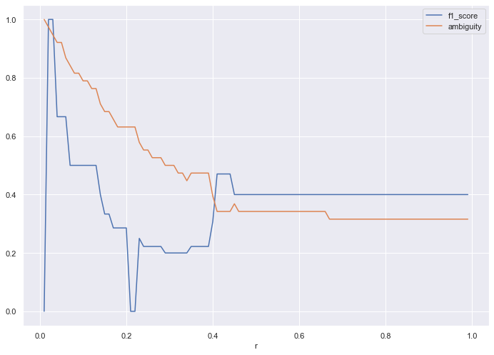
I decided to try the algorithm (keeping the ideal r) on half the training data, which results in the following loss graph:
Contrast this to the loss plot for the full training data set (from above):
Compared to the full dataset, the half dataset drives higher ambiguity, but produces a decent F1 score.
If we halve the dataset once more, (one quarter the data) we get the following loss plot.
Since we have a dearth of data, we need an r of at least 0.4 to get any traction. At that point, the algorithm produces decent ambiguity and F1 score, considering the lack of training data.
The following plot shows the RCE hit footprints given one-quarter of the training data:
Conclusion
RCE provides an interesting alternative to the more popular K-Nearest exemplar classifier. The RCE classifier learns quickly with limited training data.
Comment below if you think Tensorflow or MXNet should include this classifier in their ML libraries!