Introduction
Machine Learning engineers use Probabilistic Neural Networks (PNN) for classification and pattern recognition tasks. PNN use a Parzen Window along with a non-negative kernel function to estimate the probability distribution function (PDF) of each class. The Parzen approach enables non-parametric estimation of the PDF.
In this blog post I will discuss the following
- What is a Parzen PNN?
- Animated example of the Parzen algorithm
- Animated example of a Parzen Neural Network
- Normalization of Training Data
- Trade several approaches
- Effectiveness of approaches - Parzen vs. Nearest Neighbor
- Reduced Coulomb Energy Networks
- Descriptive Animation
- Visualization of RCE on the normalization approach
- Benefits of Ambiguous Regions
- RCE applied to the Bupa Liver disorders data set
- Conclusion
What is a Parzen PNN?
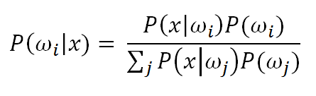
Mathworks provides a simple definition of a Parzen Probabilistic Neural Network:
The Parzen Probabilistic Neural Networks (PPNN) are a simple type of neural network used to classify data vectors. This [sic] classifiers are based on the Bayesian theory where the a posteriori probability density function (apo-pdf) is estimated from data using the Parzen window technique.
PPNN allow a non-parametric approach to estimate the required Bayesian Classifier probabilities P(x|wi) and P(wi).
In action, the PPNN mechanics are easy to follow. The PPNN takes a training vector, dot products it with the weights of the hidden layer vector and then chooses the winning class based on the highest output value. The next section includes an Animated cartoon that shows the PPNN visually.
Animated example of the Parzen algorithm
Suppose you have three classes, and the following training data:
| ID | Class | Var1 | Var2 |
|---|---|---|---|
| A | Green | 0.5 | 0.75 |
| B | Purple | 0.5 | 0.25 |
| C | Purple | 0.25 | 0.75 |
| D | Yellow | 0.75 | 0.5 |
| E | Green | 0.75 | 0.75 |
You now want to use a PPNN to classify the color of the observation ( Var1 = 0.75, Var2 = 0.25 ).
The Cartoon below shows the weights as filled colored boxes. In Column A, for example, weight one (WA1) is half full (e.g. 0.5) and weight two (WA2) is three quarters full ( e.g. 0.75). The animation shows the dot product of the test pattern ( X1 = 0.75, X2 = 0.25) with the weight vectors, an activation function, and then the selection of the winner.
Animated example of a Parzen Neural Network
Now let's take a look at the classification approach using the familiar neural network diagram. The input layer (bottom) includes our test pattern ( X1 = 0.75, X2 = 0.25), the hidden layer includes weight vectors assigned to classes based on the train patterns. The PPNN then connects the hidden layer to the appropriate class in the output layer.
Normalization of Training Data
The Mathworks PPNN web page specifies that we must normalize both our weight vectors and training vectors.
The weights on the first [hidden] layer are trained as follows: each sample data is normalized so that its length becomes unitary, each sample data becomes a neuron with the normalized values as weights w.
This next section shows different approaches to normalize the training data.
Trade several approaches
I use the following data set for this trade.
| x | y | class |
|---|---|---|
| 2.5 | 2.5 | + |
| 3 | 1 | + |
| 4 | 2 | + |
| 1 | 1 | X |
| 1 | 2 | X |
| 2 | 2.5 | X |
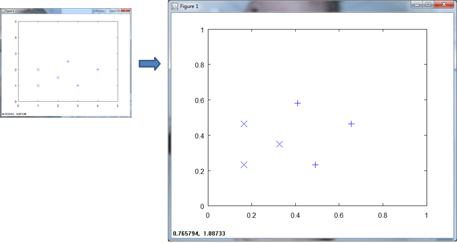
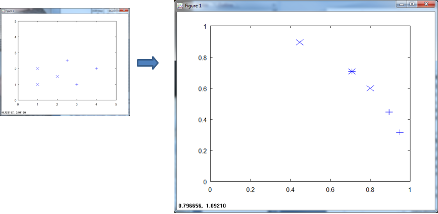
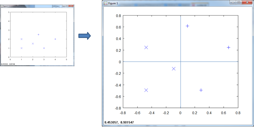
Here is a plot of the training data.
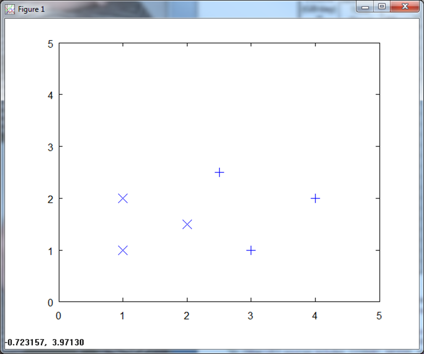
Note that in this toy example, we can set up a simple classifier via a vertical line at X = 2.25 and just use the x values to decide. Never mind that, though, since the point of this section is to illustrate different normalization techniques and then look at the effectiveness of different classification approaches.
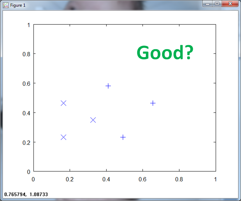
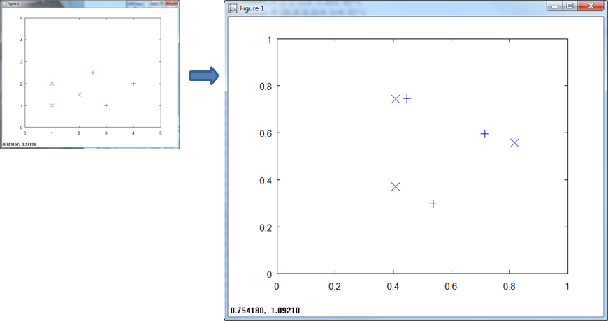
When we normalize over all the training data, you see that the (x, y) axis scale to ( 1, 1 ).
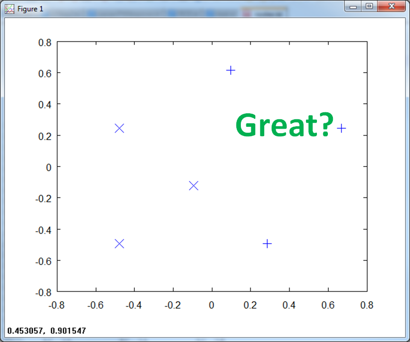
If we center the data and normalize, the scale goes from -1 to 1 on both axis.
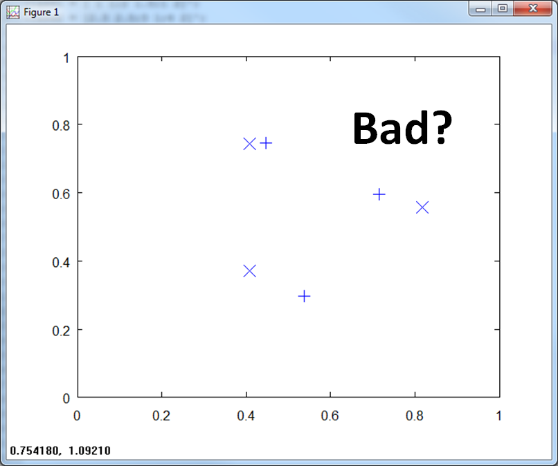
If we normalize to class specific magnitude, it makes matters worse. We no longer have clean separation of the classes.
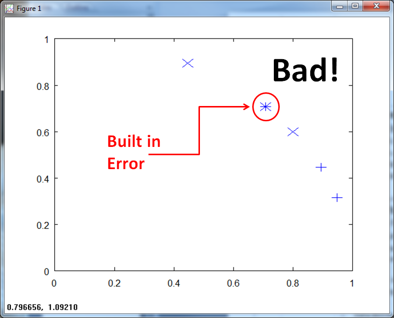
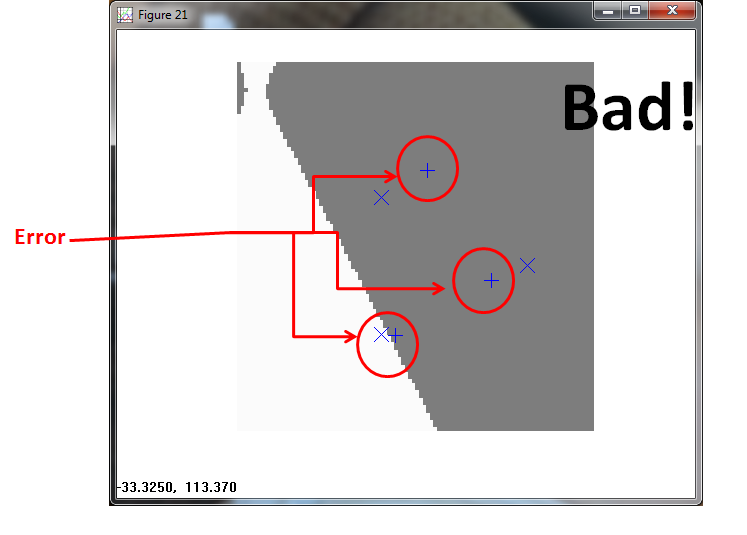
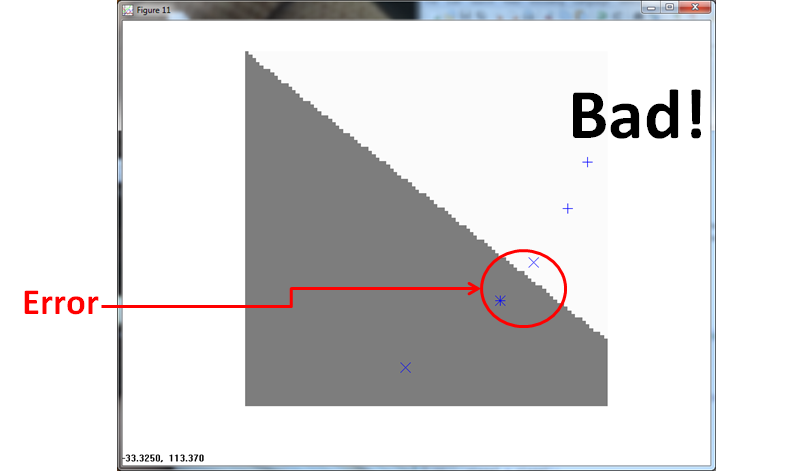
If we normalize on a per-vector basis, we get build in error. Pattern (0.75, 0.75) now belongs to both Class X and Class +.
Effectiveness of approaches - Parzen vs. Nearest Neighbor
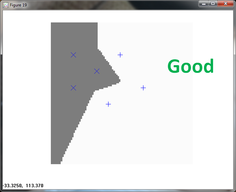
Now let's look at the effectiveness of PPNN vs. the k-nearest neighbor algorithms. KNN provides another non-parametric method of classification. Instead of using a kernel to estimate the parent PDF, it looks at the k closest neighbors of the same class. In the graphics below the gray regions depict Class One (X) and the white regions depict Class Two (+).
First lets look at the case where we normalized each training pattern to class specific magnitude. If you recall it appeared to look bad, scrunching the two classes close to each other.
KNN, believe it or not, does a good job of classifying the data.
The PPNN, fails, classifying all of Class 2 as Class 1.
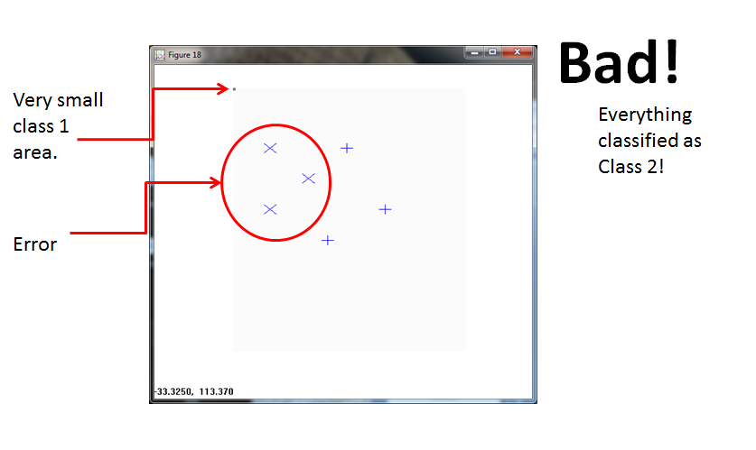
The second case scales the training data to (0,1) on both axis.
KNN handles the classification with ease.
The PPNN (using σ = 1/4 ) fails. It allocates a tiny box region to Class 1, and classifies everything else to Class 2.
Normalizing over a per-sample basis introduces built in error. Note again the overlap of the X and + at ( 0.75, 0.75).
The KNN of course takes a hit due to the build in error.
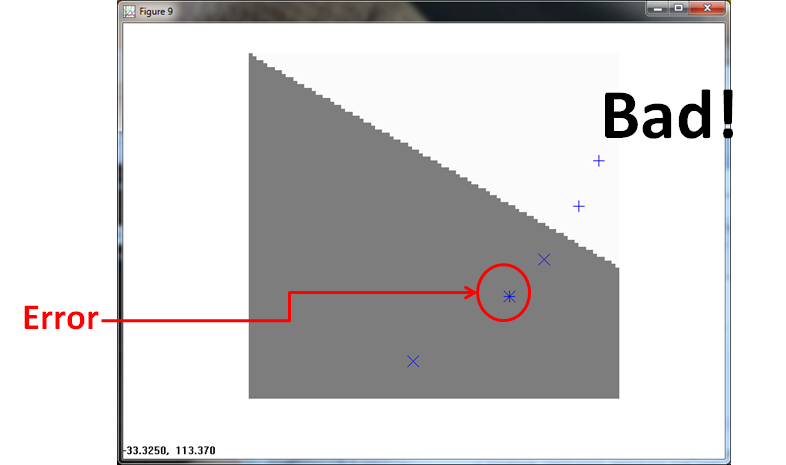
The PPNN (using σ = 1/4 ) misses twice, once for the built in error and once for a Class 1 observation.
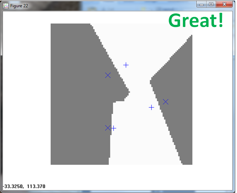
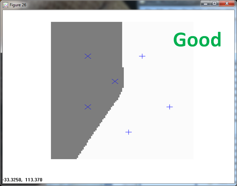
The final normalization approaches centers and normalizes the data.
The KNN handles this with aplomb.
The PPNN also correctly classifies all observations.
Reduced Coulomb Energy Networks
So far I showed several normalization approaches and then the effectiveness of different non-parametric classification techniques on the normalized data. I demonstrated, PPNN and KNN effectiveness. Now I would like to describe a third non-parametric classification algorithm. The Reduced Coulomb Energy (RCE) net.
In summary, RCE provide the following benefits:
- Rapid learning of class regions that are
- Complex
- Non-linear
- Disjoint
- No local minima issues
- Performance knobs
- Trade training time vs. memory requirements
- Trade classifier complexity to training data
If you would like more details, I encourage you to read my detailed investigation of RCE.
Descriptive Animation
This cartoon shows the simplicity of the RCE algorithm. For each training point, the RCE algorithm creates a circular footprint with a radius equal to the distance of the nearest training point from the other class. To prevent overlap, you can set a maximum radius for each training point.
Visualization of RCE on the normalization approach
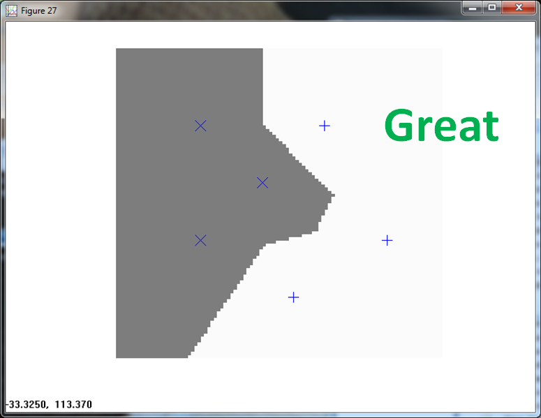
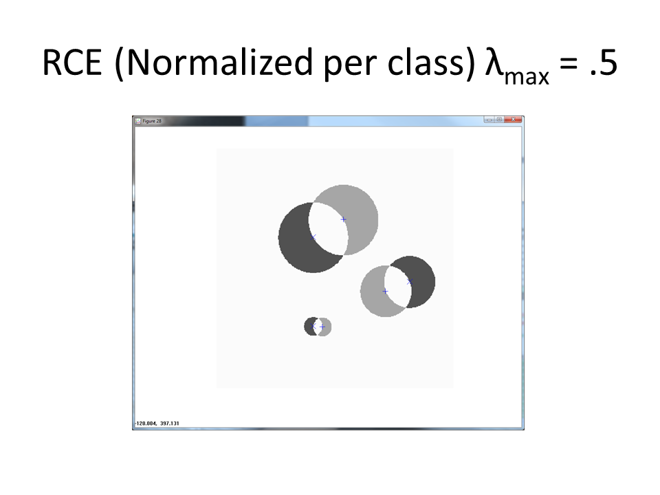
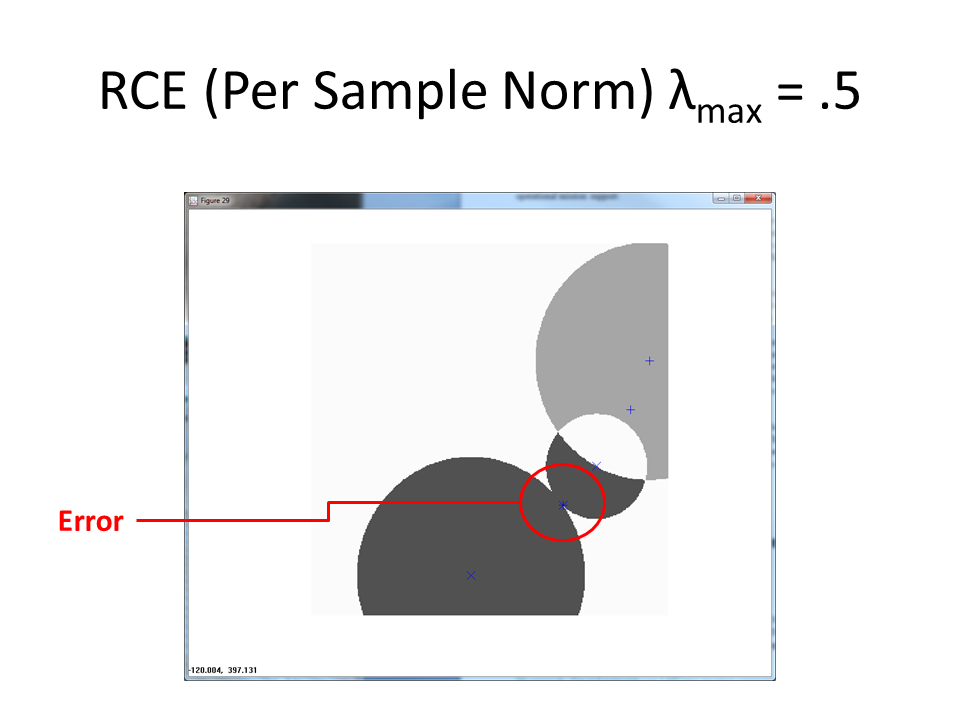
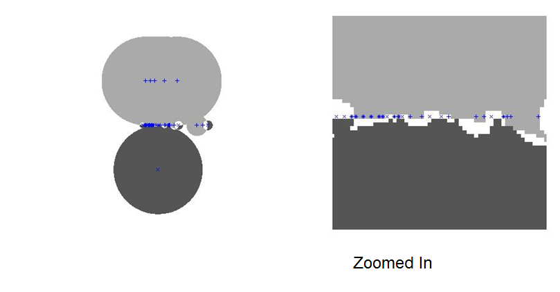
The following animation shows the classification footprints for the centered and normalized training data. Note that dark gray represents class one, light gray represents class two and white indicates an "ambiguous region" (no class).
The next animation shows the RCE classification footprints on the non-centered all samples normalized training data.
Normalized by class increases the amount of ambiguous regions.
Once more, the built in error of the normalize by per-sample magnitude approach results in a miss.
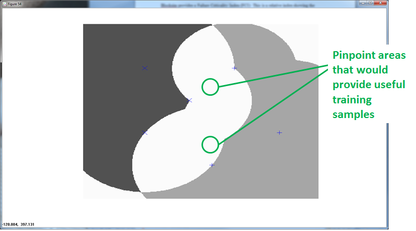
Benefits of Ambiguous Regions
RCE provides the benefit of ambiguous regions. Ambiguous regions pinpoint areas that would provide useful training samples. The data scientist can then execute observations in those regions to fill in the gaps.
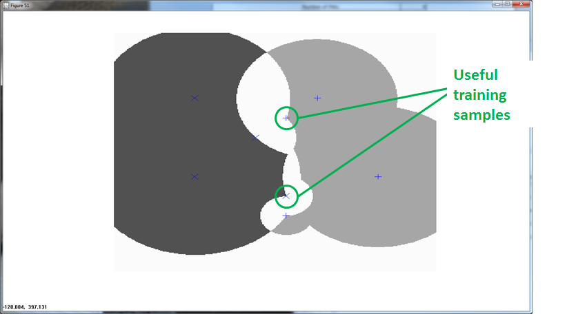
The following graphic shows how additional training observations filled in the ambiguity.
RCE applied to the Bupa Liver disorders data set
The final section summarizes my approaches to separating the training data I input into my detailed investigation of RCE.
For my investigation, I looked at the BUPA Liver Disorders data set.
The data includes six features and two classes.
- mcv: mean corpuscular volume
- Four Chemical Markers
- alkphos: alkaline phosphotase
- sgpt: alamine aminotransferase
- sgot: aspartate aminotransferase
- gammagt: gamma-glutamyl transpeptidase
- drinks # of half-pint equivalents of alcohol per day
I then wrangled the data set in order to increase the success rate of my classification. I used the following method:
- Normalize the data
- Quantify separability using
- Divergence
- Bhattacharyya distance
- Scatter Matricies
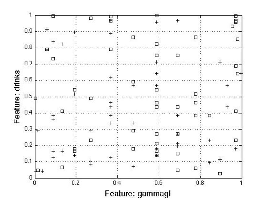
For the two feature case, separation analysis showed the best feature combination for class detection includes gamma-glutamyl and number of drinks.
Out of the box, you can see these two are poorly separable.
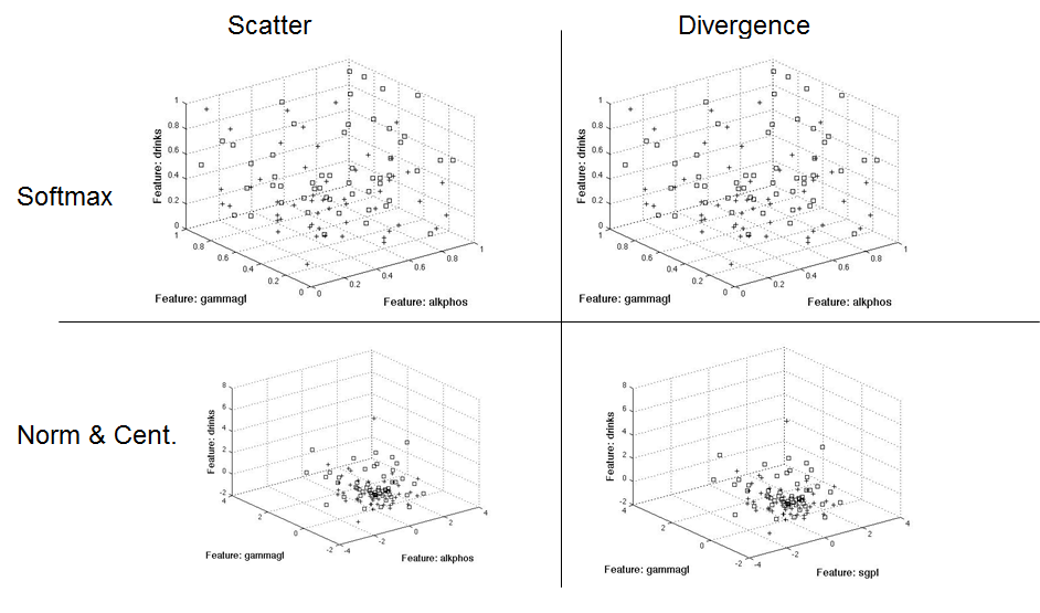
For the three feature case, the scatter method (left) added alkphos to the mix, whereas divergence and Bhattacharyya added sgpt.
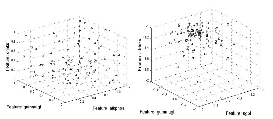
The following diagrams show the three dimensional separation approaches based on a normalized test set. I used the training μ and σ to normalize the test set.
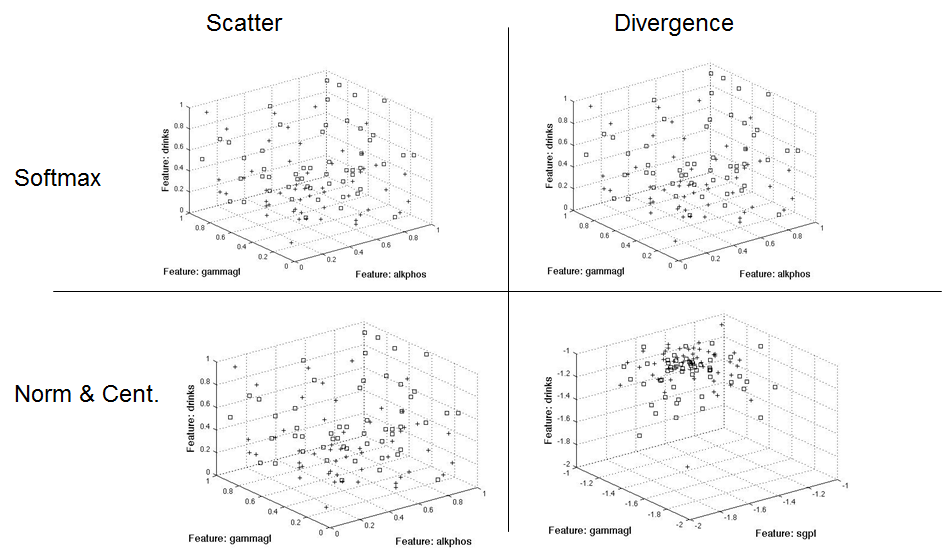
This graphic shows the same approach, only using the test set's μ and σ to normalize the test set.
The following graphic shows the classification footprints using a normalized, two feature (gamma-glutamyl and number of drinks) train and test set.
For detailed results of my investigation, I encourage you to read my detailed investigation of RCE applied to the BUPA liver disorders data set.
Conclusion
I leave you with convenient bullet points summarizing the work we accomplished today.
- Frame PNN as a simple series of steps
- Dot product (or distance)
- Non-linear transform
- Summation and voting
- Be cognizant of normalization approach
- Sometimes feature reduction yields classes with common patterns
- RCE rapidly learns class regions
- Complex
- Non-linear
- Disjoint
- RCE can ID ambiguous regions
- ID regions of useful training patterns
- Does not classify as a known class, in the case that there may be unknown classes
If you enjoyed this blog post, please check out these related blog posts: