Engineers face the reality of imperfect and noisy channels when designing digital communication systems (DCS). The engineers must account for signal degradation to ensure that a receiver receives the message that the transmitter intended.
Consider the classic kids’ game telephone, which provides a familiar example of a noisy channel. The first child whispers a message into the next child’s ear. She whispers, I would like an ice cream sandwich right now. The second kid relays this message to the next, who either due to poor hearing or creative mischief may or may not alter the message slightly. At the end of the line, the last kid relays the message to all in attendance: John Sobanski writes the best tech blog on the planet! Space to ground link terminals, radio channels, or even old disk drives represent more austere examples of noisy channels.
Engineers use two approaches to improve communication reliability on a noisy channel: Error detection and error correction. Error detection allows a receiver to flag incoming messages as corrupt. The receiver can choose to drop the flagged data or request a re-transmission.
Error detection works well on systems that use two way, or duplex communications. Clients on our modern Ethernet LAN, for example, can both send and recieve messages. For simplex communication systems, a receiver may not have the luxury of requesting a retransmission. Geosynchronous satellite communication systems, for example, use simplex communications. Real time systems, furthermore, may have a communication link available but may not have the luxury of time to send a retransmission request. In these instances, engineers use error correction to make the noisy channels more reliable (Tanenbaum 206).
Coding Theory includes the fields of mathematics and engineering that deals with making noisy channels more reliable (e.g. Bring the noise down to a theoretical lower bound of zero). Together, source coding and channel coding constitute the two main fields of coding theory. Source coding deals with compression, or the act of making a data set smaller to fit through a bandwidth limited channel. Effective compression techniques look at the probabilities of certain symbols in deciding which codes to pare from the alphabet. Source coding uses the term entropy for the fundamental measure of average information content.
For example, the English language alphabet includes 26 symbols, or characters, but some occur more frequently than others. Lexicographers have looked at millions of pages of texts to discover that the letter e occurs 171 more times than z. A source coding developer could bet that the letter z would not be present in a message containing 50 characters. He would also remove the letter q (1/126 less likely), x (1/84) and j (1/83). By using probability to hedge his bets against the occurrence of these letters, he compressed the alphabet to 22/26 its original size, or by 15%.
Coding Theorists name the above compression approach context dependent encoding. Context dependent encoding yields lossy results -- the messages lose data. Engineers deploy lossy compression to media that contains information undectectable to the receiver.
Certain messages can lose data without incident. If a receiver, for example, can't detect a certain fidelity of data, lossy compression schemes will pare these overly detailed data and the receiver won't notice. Our ears can't process certain frequencies, so the MP3 compression algorithm filters off these irrelevant frequencies to reduce the size of the final MP3 file.
Communication engineers do not apply lossy compression to data files that must retain all information without loss or edits. A bank, for example, must not lose any information contained in its customer database. Communication engineers use lossless encoding for these scenarios. Channel encoding enables lossless compression (Tanenbaum 494).
Coding Gain
DCS engineers must reliably transmit an acceptable number of bits per second through a noisy channel (B) using at most W watts. Engineers call this trade B vs. W. A transmitter, (e.g. radio station, handy talkie or satellite) has an average energy of Eb = W/B Joule per user bit available to generate a signal destined for a receiver. Coding can improve this ratio, which engineers call coding gain.
With no coding, a transmitter maps a user bit onto a signal using Eb energy. The resultant signals have amplitude s = sqrt(Eb) for a transmitted 1 and s = -sqrt(Eb) for a transmitted 0. Engineers typically model noisy channels using Additive White Gaussian Noise (AWGN), with r = s + n representing the received signal amplitude. The noise n comes from the Normal Zero mean Gaussian distribution.
A maximum likelihood receiver detects the received signal with amplitude r and makes a hard decision to label it a 0 or 1 based on the received value in relation to γ. Due to the Gaussian nature of the maximum likelihood receiver, the probability of error becomes the probability under the tail of the Normal Gaussian pdf, or Q(Eb/N0), with Q the standard complementary error or co-error function.
Eb/N0 provides the figure of merit for DCS, with Eb describing bit energy (signal power times bit time) and N0 capturing the noise power spectral density. For a codeword set M containing 2k codes, with k bits per codeword we deduce that k*Eb yields the energy per codeword. We must send the channel bits 1/k times the speed to reach the rate of B user bits per second. If we have the same constraint of W watts from before, we now only have an available energy of Es = W/k = k*Eb Joule per channel.
Inserting this information into the same AWGN channel and maximum likelihood receiver from before, our error rate per channel bit now equals Q(sqrt(k*Eb/N0)). We gain reliability, therefore, at the cost of energy per bit. For equal error probability after decoding, we call the ratio between SNR (uncoded) and SNR’ (coded) coding gain. Engineers represent the coding gain in Decibels, or 10log10(X), with X providing the reference level. For example, a coding gain of 3dB doubles the reference level, since 10^.3 = 2. (Lint 29)
To achieve coding gain, channel encoding uses variable length symbol codes, which encode one source symbol at a time. We call a collection of symbols or characters an alphabet. For a given Eb/N0, coding trades throughput for noise mitigation by adding code bits along with the error bits. When we use an n bit code word to transmit k data bits, then we have m = n – k code bits per code word. Coding Theorists named this efficiency code rate, represented by either (n,k) or k/n (Gremeny 9- 7).
Hamming Distance
The Hamming distance, d, captures the number of bits that differ between two code words. dmin >= t + 1 represents the minimum Hamming distance for detection of t errors, while the minimum Hamming distance for detection and correction of t errors requires a Hamming distance of dmin >= 2t + 1. For example, with the code efficiency of a deep space application of 1/100 coding, we have a Hamming distance of 99, and therefore can reliably detect and correct up to (99 -1)/2 or 49 errors. (Gremeny 9-10).
If two binary vectors describe the code words, then the number of coordinates where the two vectors differ yields the Hamming distance. The distance between these two vectors aid in discovering the probability we will decode in error. Decoding errors occur when noise transforms a transmitted codeword t into a received vector r, with r closer to another (wrong) codeword (MacKay 206).
How do we discover the Hamming distance? Looking at the required minimum Hamming distance for reliable correction of t errors, dmin = 2t + 1, when C has M words, we must check M choose 2 pairs of codewords to find d using brute force. We’ll find that linear codes, discussed later, require less computation, since for a linear code C the minimum distance equals the minimum weight (Lint 36).
Regardless, we realize that a large distance d between codewords results in fewer decoding errors. Mackay has quantified the metrics for good and bad distances. With codes of increasing blocklength N, and with rates approaching a limit of R > 0, then a sequence of codes has good distance if d/N tends to a constant greater than zero. A sequence of codes has bad distance if d/N tends to zero. A sequence of codes has very bad distance if d tends to a constant, i.e. it’s independent of N (MacKay 207).
Getting a qualitative feeling for the effect of the minimum distance on decoding errors proves a useful exercise. Look at a low weight binary code with blocklength N and just two codewords passing through a binary symmetric channel (BCS) with noise level f. Since we have only two codewords, the decoder can ignore any data bit positions equal for both codewords: a bit flip in those positions will not effect the probability of decoding error. The probability that d/2 of the non-equal bit positions flipped dominates the error probability. “d choose d/2” * fd/2 * (1 – f )d/2, therefore, captures the probability of bloack error.
If a block code has distance d, then it must have a block error probability of at least this, independent of blocklength N. Above, we labeled codes with d independent of N very bad. Engineers, however, have a habit of bending mathematics to get the job done. In reality, very bad codes work in practice. Consider disk drives. If we have a disk drive system with 10e-3 Pe then a codeword distance of d = 30 clocks in smaller than 10e-20. Good codes for disk drives need an error probability smaller than 10e-18, so this very bad distance suffices (MacKay 215).
Channel Coding: Block Codes
In Block encoding, we map data (message) words to code words. We encode each block of k data bits by a unique code word with a length of n data bits. We name a code that can correct up to t errors an (n,k,t) code (Gremeny 9 - 13). Additionally, we name an n-length k-dimensional linear code with minimum distance d an [n,k,d] code, or (n,M,d) with M representing the number of codewords. (Lint 35).
We need to briefly discuss some definitions to continue our discussion on block encoding. A space Rn consists of all column vectors v with n components (Strang 111). The two essential vector operations inside the vector space include (1) we can add any vectors in Rn and (2) we can multiply any vector by any scalar (Strang 112). A subspace of a vector space includes a set of vectors, including 0 that satisfies two requirements. If we have two vectors v and w in the subspace and any scalar c, then the subspace includes both (i) v + w and (ii) cv (Strang 113).
A message vector contains each block of k message digits, and a code vecor contains each block of n codeword digits. Linear block codes map message vectors onto codeword vectors. For binary block codes, we have a one to one assignment from each of the 2k distinct message vectors to separate and unique code vectors. We call the set of all possible code vectors the vector space. We therefore can select 2k vectors from the pool of 2n potential code vectors to represent the necessary 2k message vectors. We call this selection a subspace of the vector space, and it must adhere to the definition for subspace above.
With alphabet Q representing the n dimensional vector space, we define the subspace C of Qn to contain the collection of code vectors. Communication engineers name a k by n matrix whose rows provide a basis of liner code C a generator matrix G (Lint 35). The generator matrix allows us to only store the k rows of G instead of having a lookup table of size 2k in memory. We can form any of the necessary 2k code vectors by multiplying a message row vector by the generator matrix.
We consider a code C systematic on k positions if |C| = 2k and we have one codeword for every possible choice of coordinates in the k positions. We call the symbols (1 or 0 for binary) in these k positions information bits (Lint 36). Any [n,k] code, must prove systematic on at least one k-tuple of positions. In other words, a systematic linear block code generator matrix maps a message vector onto a code vector such that the resultant code vector contains the original message vector plus m additional bits.
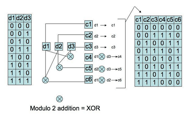
A systematic linear block code generator matrix has the form G = [ P | Ik ]. We call P, the first part of matrix G the parity matrix. From this we can create the parity-check matrix H = [ In-k | PT ]. We use H to create the syndrome test matrix S = rHT, with r a received code vector. The syndrome test matrix produces a syndrome. We have a coset on hand that maps all expected syndromes to error patterns. Once we lookup the error pattern for a given syndrome, we add it to the received vector at which point modulo 2 addition will correct the error (Sklar 333).
Conclusion
In this blog post we discused noisy channels, coding gain, hamming distance and block codes. Next month we will deep dive into Convolutional codes.
If you enjoyed this blog post, you may be interested my discussion of a Discrete Event Simulation (DES) for Adaptive Forward Error Correction (AFEC).
Otherwise, be sure to proceed to part 2.
Bibliography
- Gremeny, Steven E. Ground System Design and Operation. Chantilly, VA: Applied Technology Institute, 2003.
- Lint, J.H. van. Introduction to Coding Theory Third Edition. Eindhoven, Netherlands: Springer, 1991.
- MacKay, David J.C. Information Theory, Inference, and Learning Algorithms. UK: Cambridge University Press, 2003.
- Sklar, Bernard. Digital Communications: Fundamentals and Applications (2nd Edition). Upper Saddle River, NJ: Prentice Hall, 2001.
- Strang, Gilbert. Introduction to Linear Algebra Third Edition. Wellesley, MA: Wellesley-Cambridge Press, 2005.
- Tanenbaum, Andrew S. Computer Networks Second Edition. Englewood Cliffs, NJ: Prentice Hall, 1989.