Over the air communications, such as text messages, satellite radio, walkie talkies and WiFi need to deal with the unpredictable effects of noise in the channel. Coding theory attempts to make noisy channels more reliable by bringing the noise down to a theoretical lower bound of zero. Channel coding, as opposed to source coding, provides a lossless method of reducing noise.
Part One of this blog series discusses the use of Block Codes in channel coding. This blog post discusses channel coding via the use of Convolutional codes.
Channel Coding: Convolutional Codes
Convolutional codes produce n code bits in response to the k input bits from both the current time unit and the previous N-1 input data bits. We refer to convolution codes as (n,k,L), with n and k equal to output and input bits respectively. We define L, the constraint length, as L = k(m-1), with m equal to the number of memory registers. The figure below describes an encoding device:
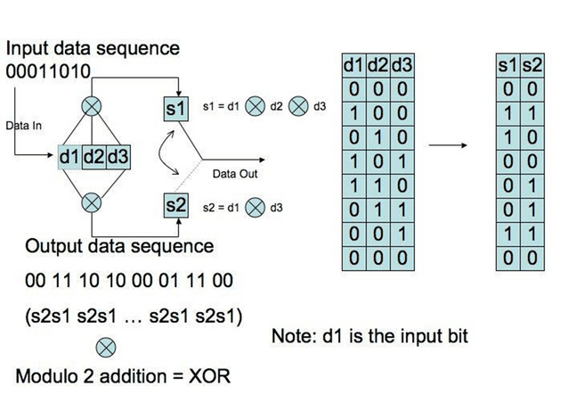
The constraint length is 3, with n=2 output bits. Squares d1, d2 and d3 represent the flip-flops that can be in either state 0 or 1. They are connected to modulo two adders to represent the generator polynomial. An external clock produces a signal every t0 seconds (assume t0 = 1), causing the contents of the flip-flops to move to the right (i.e. a shift register). The modulo 2 operations produce the output bits s1 and s2 (Lint 181).
Mathematically, if we describe the input stream i0, i1, i2, … as a power series I0(x) : = i0 + i1x + i2x2 + … with coefficients in 2 dimensional space, describe the outputs at s1 and s2 as T0(x) and T1(x) and synchronize the external clock so the first input corresponds to the first output then, for the polynomials 1 + x2 and 1 + x + x2 we get T0(x) = (1 + x2)I0(x) and T1(x) = (1 + x + x2)I0(x).
We interlace the outputs as T(x) = T0(x2) + xT1(x2). For example, if we had an output stream 11 01 11 00 00 …, G(x) := 1 + x + x3 + x4 + x5 = (1 + (x2)2) + x(1 + (x2) + (x2)2). Defining I(x) := I0(x2) T(x) = G(x)I(x). We refer to the polynomial G(x) as the generator polynomial of this code (Lint 184).
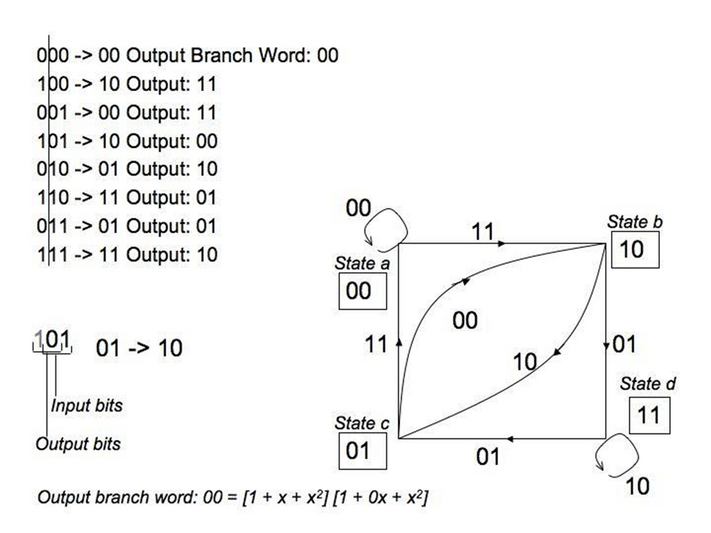
Lint prefaces the previous diagram with “every introduction to convolutional coding seems to use the same example. Adding one more instance to the list might strengthen the belief of some students that no other example exists, but nevertheless we shall use this canonical example (182).” Most of my sources included this diagram, and the state diagram that follows, yet despite its ubiquity I did not find a clear explanation as to how the latter followed the former. For that reason, I decided to look at the problem until I could describe it to a layperson. The state diagram is actually quite simple.
The key is to understand that only the right two flip-flops in the diagram are the memory registers, the first is the input. The two memory registers can be one of four values, 0 through 3 (in binary). If they are at 00 for example, the input bit can only be a 0 or a 1. If it is a 1, we get 100 and the output bits are 11 from the polynomial. Then, when the shift register moves the bits, the memory registers are now 10. Going back to 00 in the memory register, consider an input bit of 0. The three registers are now 000, which applying the modulo 2 adders gives us an output of 00. The shift register then shifts the two zeros to the right into the memory registers. Therefore, if start at state 00, we can only transition to state 10 (with an output of 11) or stay at state 00 (with an output of 00).
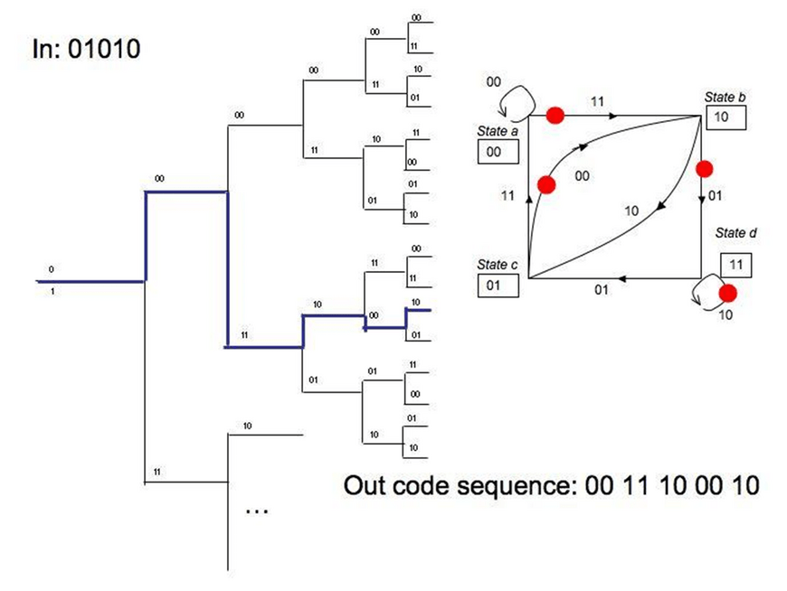
Another representation of convolutional encoding is the tree diagram, which attempts to show the passage of time as we go deeper into the branches. Instead of moving from one state to another, we go down the branches of the tree whether a 1 or 0 is received. If we receive a 0, we go up a branch. If we receive a 1, we go down a branch.
The first two bits show the output bits, and the number in the parenthesis shows the operation of shifting in the input bit, or the output state (Langton 12). The tree diagram is not the preferred diagram for engineers. In the diagram below, the state diagram is added for reference, with the 1 input bits highlighted by a red circle:
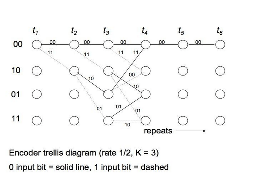
The preferred method is the Trellis diagram. We draw all states on the y-axis. The x-axis represents discrete time intervals. When we receive a 0 we go up using a solid line, for a 1 we use a dashed line flowing down. On the line we write the output, or the codeword branch. After L bits, all states are reached, and the diagram repeats. Coding is easy with a Trellis diagram, for an input string, we merely go up for a 0 bit or down for a 1, and copy down the codewords along the path.
Channel Coding: Decoding convolutional codes
The decoding of convolutional codes almost resembles the decoding of block codes since we’re comparing the received word with all codewords. Convolutional codes, however, have infinitely long codewords so the receiver must only look at the first l symbols of the received message (Lint 185).
Convolutional decoding, therefore, deals with decoding sequences of length s without having to check every one of the possible 2s codewords. The two main types of convolutional decoding are sequential decoding (Wozencraft and then Fano) and maximum likely-hood decoding (Viterbi). We will look at the Viterbi algorithm here.
Viterbi implements maximum likely-hood decoding by reducing the options of a Trellis path at each time tick. When a decoder receives a branch code that is not possible for the current state, it simultaneously calculates two separate paths and assigns each Hamming metric. At any given time tick t, the trellis has 2L-1 (L = constraint) states, and each state can be entered by one of two paths.
The key to Viterbi decoding algorithm is to assign metrics to each of the paths and sloughing off one of them. The winning path is known as the survivor. The Viterbi algorithm uses these principles (1) That errors occur infrequently and the probability of error is small and (2) The probability of burst errors is much less than that of a single error (Langton 21).
Conclusion
FEC using either block or convolutional codes trade bandwidth for a lower bit error rate for fixed power. Communication can be simplex and real time, but the receiver must decode and correct errors. Block codes operate on blocks of bits. We break a chunk of data up and add error correcting bits to it. Convolutional codes are continuous, and operate on bits continuously.
If you enjoyed this blog post, you may be interested my discussion of a Discrete Event Simulation (DES) for Adaptive Forward Error Correction (AFEC).