Satellite system engineers consider the narrow beams (which lend themselves to frequency reuse) and high data rates of Ka band channels attractive for communication systems [Khan 2]. As a result, the satellite community witnessed a great increase in the number of Ka band Satellites over the past two decades. During this time period, Satellites have moved from low rate backup systems to critical Internet service provider (ISP) hubs and real time dissemination nodes. We see that satellites have increased in criticality while embracing a wavelength that is susceptible to atmospheric loss. This combination has lead to new methods for gain. This paper discusses one such method, coding gain using Adaptive Forward Error Correction (FEC). The outline of this paper follows. First I will discuss AFEC, to include the effects of encoding choices, detection (fade prediction) schemes and finally the necessity fade detection margins. Then I will describe a numeric MATLAB simulation that investigates the gain associated with AFEC techniques, and the role that prediction time plays in gain.
What is AFEC?
A critical parameter for satellite communications systems is availability, which describes how often the link can transmit or receive data [Gremont 1]. Digital systems objectively describe this measure as bit error rate (BER), or the average number of bit flips a string of digital data can expect traversing a channel. Another way to describe BER is Eb/No, or the average energy per bit to noise spectral density [Yang 368]. In other words, how much Eb/No does a channel require to maintain an average BER? A system may require, for example 10 dB of Eb/No to maintain a BER of 1e-6, or 97% availability.
Severe rain activity from thunderstorms greatly attenuates Ka band links and therefore can lower availability. Thunderstorms do not have a uniform distribution; they are rare but severe events [Khan 10]. Due to the criticality of most Ka band links, system engineers nonetheless must account for these severe but infrequent events [Khan 10]. Khan demonstrates a system that must increase Eb/No from 10 dB to 20 dB in order to see an availability increase from 99% to 99.9% [Khan, Figures 1 and 2]. In general, we can reduce BER by trading power, bandwidth or transmission times. Unless absolutely necessary, site diversity would be untenable, due to the monetary cost. For TDMA, power and bandwidth are fixed [Khan 11], so we trade on transmission time by consuming slots to provide gain in the form of redundancy. Forward error correction (FEC) provides this redundancy and therefore gain, which we refer to as coding gain. With FEC gain, for example, the previous system could possibly require only 7 dB for 99% availability. The issue with FEC is that it requires redundant bits to reliably encode data, therefore lowering data throughput. The parameter code rate describes the effect of coding on data throughput and is the fraction of useful information that can pass through a channel. The disadvantage to FEC coding for gain against rare events “is that bandwidth will be wasted when the channel is in a ‘good’ condition, which may occur most of the time” [Yang 368].
Adaptive FEC (AFEC) minimizes wasted resources by applying different intensities of code depending on the channel loss [Khan 9]. An appropriate AFEC scheme requires an engineer to select the optimal coding method, code rates, number of states, attenuation thresholds for each state and fade prediction (detection) algorithm. Each situation is unique, and as Khan writes, “the criteria to select an ideal AFEC scheme are quite contradictory in nature and impossible to satisfy all at the same time” [Khan 12]. The goal is to have the proper amount of FEC relative to the amount of channel degradation [Khan 12]. Too much or too little either allows error to go uncorrected, or wastes resources (I discuss this further in the section on detection schemes below).
An AFEC system nonetheless has attenuation thresholds based on the number of states (codes). Consider a two state system. The AFEC system detects the Eb/No in the channel. If the channel crosses the attenuation threshold, it applies the low code rate (high FEC tax) encoding scheme. If the channel crosses the threshold back to the normal Eb/No, it switches back to the high code rate FEC scheme. As an example, for Khan’s system “a suitable rain countermeasure scheme may be realized by having a fixed fade margin of 11 dB and two levels of adaptive resource sharing to achieve an additional 5 dB for about 1% of the time and 9 dB for about 0.5% of the time [Khan 10].” I discuss the notion of a fade margin further below.
Which encoding type should I use?
Since fade events are infrequent, the low gain code will be used for the vast majority of time. The efficiency of the low gain code, therefore, drives the “average delay” number for the AFEC system, since it accounts for a very high proportion of the “average delay” sampling period. AFEC systems, furthermore, are sometimes applied to channels with a high number of end users, each with their own receiver. Cost and low complexity are huge factors in this case, since consumers will not spend thousands of dollars on expensive decoding equipment. In order to reduce complexity and therefore increase customer adoption, therefore, a system engineer needs to pick a code that is efficient and inexpensive to implement as both a high gain, and (especially) a low gain code. Khan recommends that the high gain code implement the same encoding scheme as the low rate code [Khan 12-17]. He specifically recommends a double encoding scheme using a high and low rate Golay code. “The double coding AFEC scheme, using Golay code, has a moderate [total coding gain] TCG (5 dB and 8.1 dB) with little coding/decoding delay. The Golay codes are simple to implement and suitable for high-speed operation” [Khan 17 & Table III].
Satorius also investigates encoding approaches and demonstrates how the proper combination of (A)FEC schemes along with optimal encoding methods results in higher coding gain and higher channel efficiency. He begins with a static ½ convolution code and demonstrates how the addition of AFEC with a second ¼ convolution code state provides an additional coding gain of 4 dB. That is, in order to maintain an average BER of 1e-6, the “two state” AFEC approach requires 4 dB less Eb/No. Satorius then describes how keeping that 4 dB in the system along with AFEC increases the channel availability from 97% to 98.7%. Keep in mind that the Eb/No to availability graph hits a knee at about 97% [Khan 10, figure 1], so this increase is significant. Furthermore, for the AFEC scheme he calculates the average coding rate over a Raleigh fading channel as 48%, which is just a slight penalty compared to the fixed rate ½ code channel. He increases the coding gain another 3 dB by replacing the convolutional codes with ½ and ¼ rate turbo codes, keeping the coding rate at 48%. If we maintain the same Eb/No as the static ½ convolutional FEC scheme, we increase the channel availability from 97% to 99.4%, an 80% reduction in channel outages. Using 7/8 and ¼ punctured turbo codes increases the coding gain another 2 dB and increases the average coding rate to 80%! [Satorius 324-325]
Yang supports Satorius’ acclaim for an AFEC scheme using punctured turbo codes. He writes “high rate punctured convolutional codes and maximum distance separable (MDS) block codes are particularly well suited to implement the adaptive FEC encoder and decoder [Yang 369].
Which Fade Prediction methods do I use?
What separates AFEC from static FEC is the adaptation of coding intensity to channel degradation, which requires detection of the current Eb/No. For AFEC, “monitoring the received power or bit error rate (BER) to detect the occurrence and magnitude of rain fade is required” [Khan 11]. Rain events, while rare, may fluctuate rapidly and therefore, “to cope with the rapidly changing link degradation (0.1 to 0.5 dB/s) detection and allocation of countermeasure has to be affected very quickly” [Khan 11]. The effectiveness of an AFEC scheme is “conditioned greatly by the ability of practical [fade counter measure] FCM controllers of detecting and predicting the actual level of the total attenuation on a satellite link” [Gremont 1]. Accurate fade detection raises availability since “matching channel conditions more closely via a multi-rate system yields even better average system throughput while maintaining the desired availability” [Satorius 326]. One method of fade detection uses a closed loop. Some closed loop systems, however, have a large round trip time (RTT) that causes the measurements to reach the detector after a delay, which necessitates prediction.
Fade prediction can either be long range or short range. Closed loop systems with long propagation delays, such as bent pipes from GEO satellites use long range prediction. Open loop systems do not have the feedback delays and thus use short term prediction. Since a GEO satellite has a RTT of ~0.25(s), the long-range prediction must compensate for this delay. [Satorius 321-322]. Satorius provides an overview of long-range prediction methods based on least-squares modeling and short term block analysis using a “signal sub-space based algorithm” that “enables rate adaptive transmission techniques over bent pipe paths, especially when the de-correlation time of the scintillation is in excess of 0.5 secs” [Satorius 322]. Satorius points out how the sampling rate must be considered carefully, since it affects the quality of the prediction, which in turn drives the average throughput achievable by the AFEC system. He provides a situation where a fade sampling rate of 80Hz produces prediction quality degradation in the presence of “deep nulls,” where a sampling rate of 8Hz does not [Satorius 323].
How much margin is necessary?
Fade detection, while critical, is not a perfect art. “Even if the fade data are known exactly, there will still be errors associated with the prediction process” [Satorius 322]. Fade counter measure (FCM) systems may underestimate or overestimate fade events. Underestimation of fade results in high bit errors, whereas over estimation wastes resources and channel capacity. Systems engineers, therefore, must account for fade estimation errors in the form of fade detection margins. Gremont provides a table that lists the required fade detection margin (FDM) to achieve a specified percentage link availability, given a time delay in seconds [Gremont 5, Table I], with the delay being how far ahead a FCM needs to predict a fade event.
Simulation
For my project, a finite state machine (FSM) simulates the AFEC environment. The FSM simulates the noisy channel with and without fade events, and the correction probability for both high and low code rate FEC. In addition, the FSM contains a detection portion that toggles between the two FEC based on detected error rates. In order to investigate internals, I have created this simulation ”from scratch,” only using MATLAB functions for the “non FEC" portions, such as Matrix operations and probability density functions. The next sections describe the error model, the correction probability model and then the AFEC system model.
The Error Model
The AFEC FSM contains both high and low code rate FEC. Since they share a lowest common denominator (LCD) I selected a 57/63 ( η= 0.9048) code for the high code rate FEC and a 4/7 (η = 0.5700) code for the low code rate FEC. The model uses a linear block encoding scheme based on Hamming [Lint 33-38] (see next section: “correction probability model”). The error model uses the binomial distribution based on number of bits per block. For example, assuming a fade event BER of 1e-2, the probability that one bit in a 63 bit high code rate FEC block flips equals (63 choose 1)*(1e-2)1*(1-e-2)(63-1). I limited the BER model to a maximum of 7 errors per block, and created matrices of error probabilities using the MATLAB binopdf function:
BIT_ERROR_MATRIX = binopdf(1:7,BITS_PER_BLOCK,BIT_ERROR_RATE)
This produces an array with each index holding the probability of bit error for index errors per block; that is, BIT_ERROR_MATRIX(3) holds the probability of 3 errors for a 63 bit block passing through a channel with a 1e-2 BER. For example:
binopdf(l:7,63,le-2) = [ 0.3378 0.1058 .0217.0033 .0004 3.8e-5 3.2e-6]
The ber_model.m script uses these arrays to calculate the number of hits per FSM iteration. The script generates a random number 0 <= r <= 1 and then matches r to the bit error array and returns the number of hits. For the array above, a value of r = .005 returns 3 hits.
The Correction Probability Model
The correction probability model pseudocode follows:
- Generate a block
- Calculate and apply BER hits (if any)
- Calculate syndrome
- Select and apply error vector based on syndrome
- Compare repaired block to generated block
- Update bits sent, bits in error and repair success counters
The correction probability model follows linear block encoding via Sklar (pages 333-341), and begins with block generation. To save compute resources, the model only generates a block if there are hits present, assuming that a block received without errors will be decoded successfully. The model investigates the low code rate FEC with 7 bit block size. Our generator matrix, therefore, is G = [P eye(4)] which concatenates the (4,3) parity matrix (selected as P = [111;110;101;011]) with a (4,4) identity matrix. The Hamming matrix is a (3,3) identity matrix concatenated with the transpose of the parity matrix, or H = [eye(3) P’]. The code then generates a random (1,4) vector d and multiplies it by the generator matrix to send the encoded vector U. The error model randomly flips bits on this vector (i.e. applies error vector e), and produces the vector r = U + e. The model calculates the syndrome via r*H’ to produce vector s. The model selects all error vectors with syndrome s. The model then picks the error vector with the least Hamming distance between vector r and vector (r+e).
I produced the syndrome lookup table using MATLAB, which is in the appendix under syndrome_lookup_generation.m. I first create a (128,7) Matrix whose rows contain the row number in binary, that is, e = [0 0 0 0 0 0 0; 0 0 0 0 0 0 1; 0 0 0 0 0 1 0 ; 0 0 0 0 0 11 etc.]. Then I multiply this matrix by the Hamming matrix to produce a (128,3) matrix of syndromes. I multiply this matrix by the vector [4 2 1]T to create a vector of decimal syndromes. This vector S indexes the syndromes of the error matrix. For example S(27) = 3, which means the 27th error vector in e has a syndrome of 3 (we can verify this since mod(e(27,:)*H',2)*[4 2 1]’= 3 ). The MATLAB command e(S==3) pulls all error vectors from e that have a syndrome of 3. Not surprisingly, for any of the eight possible syndromes, this matrix (e_lookup) has a length of 16. The correction probability model takes this matrix, e_lookup and adds each vector to the received vector. The model keeps the resulting vector that has the shortest Hamming distance from the received vector as the repaired vector. The model then compares the repaired vector to the transmitted vector and tallies the counters as laid out in step 6 above.
The results from this investigation follow. I have not investigated the high rate code using this model, since it would require a lookup table with 263 = (~1019) entries.
| Hits Per Block | 1 | 2 | 3 | 4 | 5 | 6 | 7 |
|---|---|---|---|---|---|---|---|
| Occurances | 232130 | 84027 | 18356 | 2799 | 331 | 38 | 4 |
| Failed Repairs | 0 | 72261 | 8904 | 2446 | 213 | 33 | 4 |
| Repair Success | 100.00% | 14.00% | 51.49% | 12.61% | 35.65% | 13.16% | 0.00% |
The AFEC System Simulation
The key to Adaptive FEC is to match the power of the coding to the amount of loss. The tradeoff is that the extra coding reduces efficiency. A system designer needs to ensure that AFEC applies extra coding only when the system contains enough errors to warrant the extra coding. Additionally, if AFEC does not apply proper coding during high loss events, then the system will suffer errors. An AFEC system must balance the efficiency of the channel against the proper amount of coding necessary to mitigate against loss. An important part of any AFEC system, therefore, is to properly sense the amount of loss in the system.
My AFEC simulation contains a FSM with four states. The channel can be experiencing a fade event and thus great loss, which I refer to as the state of being in “High BER.” The channel can be outside of a fade event and experiencing normal loss, which I refer to as “Low BER.” If the encoders apply a large amount of FEC (that is, they have a low code rate), they are in a state of “High FEC.” If they apply a low amount of FEC (they have a high code rate), they are in the state of “Low FEC.” Thus, either the encoder FEC rate matches the BER or it does not. The four states are “Low FEC Low BER (Match),” “High FEC High BER (Match),” “Low FEC High BER (Mismatch),” or “High FEC Low BER (Mismatch).”
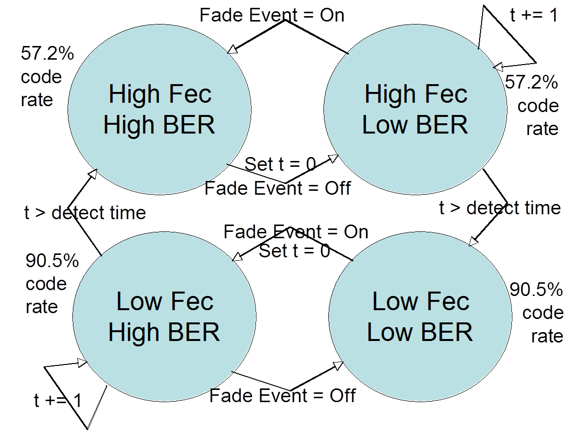
The goal of the system, therefore, is to be in one of the two “match” states, “Low FEC Low BER” or “High FEC High BER” as much as possible. The key to leaving the mismatched states is the detection time. Consider the system applying low FEC during a low BER period, which is ideal. If a fade event occurs, the FSM is now in the “Low FEC High BER” state, and experiences high loss. The FSM must wait until the detection time passes in order to switch to the desired “High FEC High BER” state. This detection time, for example, can be based on the round trip time to a GEO satellite, which is approximately 250ms.
The MATLAB simulation contains a switch statement that jumps to the current state. Each state executes the appropriate BER model to calculate hits (based on if there is a fade event or not) and the probability of repair success (based on the FEC rate used). Each state checks for state transition. For example, a fade event causes a state transition from a low BER state to a high BER state and cessation of the fade event causes the reverse. The expiration of the detection timer toggles the amount of FEC application.
Parameters
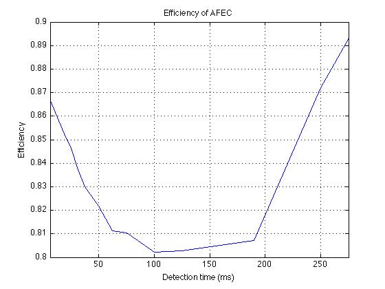
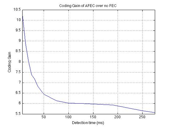
The MATLAB file sim_header.m contains the parameters used for the simulation. For the high FEC (low code rate) I used a 4/7 linear block code and for low FEC I used a 57/63 linear block code. The code used drives the error model as described in the error model section above. In addition, the code used drives the repair success model as well. In order to save computation cycles I generalized that the 57/63 code can repair at most 1 bit flip and the 4/7 code can repair at most 2. For a fade event, the probability of error is very high at 1e-2, and during normal operations only 1e-6. I use 1e-6 for the clear sky BER, since it is recommended “by the International Radio Consultative Committee (CCIR) as standard for… data transmission” [Khan 11]. The probability of a fade event toggling on or off during any iteration of the model is set at 1e-2. The detection time varies, which I explain below. The simulation calculates the total number of bits sent, the number of hits and the number of failed repairs. The simulation converts the ratio of hits to bit sent to Decibel, and does the same to the number of failed repairs. The difference of the two is the coding gain. In terms of efficiency, the simulation keeps track of the proportions spent in either the high FEC or low FEC state. Not surprisingly, the system is more efficient and produces more gain when the detection time is low since the FSM will get to one of the two ideal states more rapidly. The simulation results point to the utility of the predictive fade detection techniques, as mentioned in the first section of this paper.
Results
I wrote a script that runs the simulation five times for each of fourteen parameter sets and averages the resulting efficiency and Coding Gain. Each simulation execution iterates 1e6 times. For the fourteen parameter sets, I used the following static parameters: The channel during a clear day has a BER of 1e-6. The channel during a fade event has a BER of 1e-2. Finally, the probability of the channel going into and out of a fade event is 1e-2. I varied the detection interval, from t = 0 to t = 1100 (with t = 1 = 25μs). The results follow.
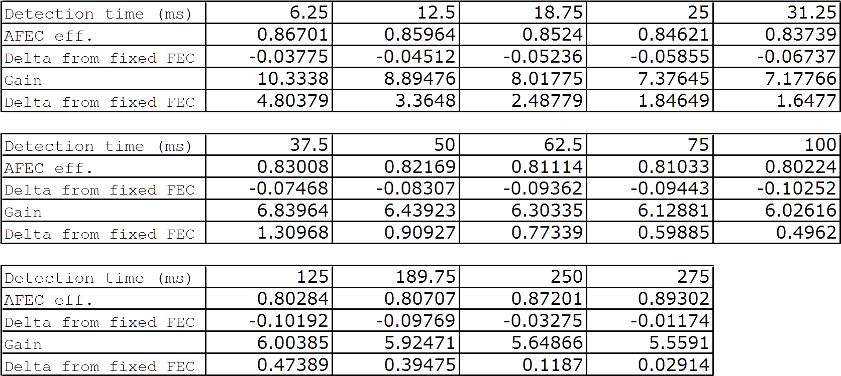
What this tells us is that as t approaches zero, we see an increase in coding Gain over both no FEC and static FEC, as well as efficiency. As t approaches infinity, the parameters converge on the static FEC case, of 57/63 efficiency and a gain of ~5.53. Graphs of the data follow.
Conclusion
Forward Error Correction (FEC) increases the reliability of data transmission over a link by adding redundant information to a transmission that receivers downstream use to repair or recreate any damaged or missing data. FEC, however, works best when the link’s error probabilities are known or at least reasonably consistent. Rain attenuation events, however, cause severe data loss to a communication channel, several deviations away from the normal data loss. The FEC rate used for a channel during non-rain (normal) communications, therefore, may not suffice during rain events. At the highest level, Adaptive Forward Error Correction (AFEC) tunes the amount of redundancy to mitigate the channel loss at hand. AFEC must find the optimal redundancy, because too much redundancy may exacerbate the situation by overwhelming the receiver with redundant data, instead of useful information. This paper described the mechanisms involved in deploying a successful AFEC system to include encoding type, attenuation thresholds, number of states, fade detection margin and most importantly (for closed loop GEO systems) fade prediction methods. In addition, this paper described the finite state model created by the author for this paper that performed numerical simulation to investigate the effects of prediction delay on AFEC utility.
Code
I posted all of my custom developed code to GitHub.
You can download it here.
Bibliography
Gremont, B., Filip, M., Gallois, P., Bate, S. Comparative Analysis and Performance of Two Predictive Fade Detection Schemes for Ka-Band Fade Countermeasures. IEEE 1999.
Khan, M.H, Le-Ngoc, T., Bhargava, V.K. Further Studies on Efficient AFEC Schemes for Ka-Band Satellite Systems. Lakehead University: IEEE Transactions on Aerospace and Electronic Systems, Vol AES-25, No. 1, Jan 1989.
Lint, J.H. van. Introduction to Coding Theory Third Edition. Eindhoven, Netherlands: Springer, 1991.
Satorius, E.H., Ye, Z. Adaptive Modulation and Coding Techniques in MUOS Fading/Scintillation Environments. JPL Pasadena, California: 2002.
Sklar, Bernard. Digital Communications Second Edition. Upper Saddle River, NJ: Prentice Hall PTR 2001.
Yang, Qing, Bhargava, Vijay K. Performance Evaluation of Error Control Protocols in Mobile Satellite Communications. Victoria, BC: IEEE 1992.