Last month, I refactored a custom Artificial Intelligence (AI) algorithm from Pandas to Polars. This switch drove a 25x increase in performance.

I needed to change the logic from a row-based apply approach to a holistic, matrix-level join/ GROUP BY approach.
My algorithm, however, experienced an Out Of Memory (OOM) error when I attempted to train a corpus of twenty-seven million (27M) observations. I then discovered the Streaming feature of Polars, which solves this issue.
Polars Streaming parallel processes in the time domain. It chunks data into memory, spreads the computation across all cores, saves the result, and loads the next chunk. This way, you can perform Big Data operations on a meager Collab notebook.
Recap: The Algorithm in Polars vs. Python
The exemplar, Reduced Columb Energy (RCE) algorithm works like the familiar k-nearest algorithm with a subtle twist. RCE calculates a hit footprint. The distance to the closest observation of a different class defines the hit footprint radius. The math then calculates the distance to every other observation of a different class. The class of each observation with a distance less than the hit footprint radius yields a hit for that class.
The original Pandas approach uses the following Lambda function to implement the logic.
def find_hits(df, v, outcome ):
  return (( np
            .linalg
            .norm(df
                    .loc[df['outcome'] == outcome]
                    .iloc[:,:-2]
                    .sub(np
                           .array(v)),
                  axis = 1)
             < df.loc[df['outcome'] == outcome]['lambda'] ).sum() )
I then apply the lambda function to each row.
The Polars approach uses columnar/matrix-based operations.
squared_distance_expr = sum(
    (pl.col(col) - pl.col(f'{col}_other'))**2 for col in princomp_cols
)

df_with_other_outcome = df_with_other_outcome.with_columns(
    squared_distance = squared_distance_expr
)

group_cols = [
    col for col in df_with_other_outcome.columns
    if col.startswith('princomp') and not col.endswith('_other')
] + ['outcome']

min_squared_dist_polars = (df_with_other_outcome
    .group_by(
        group_cols
    )
    .agg(
        pl.col("squared_distance")
        .min()
        .alias("min_squared_distance")
    )
)

lambda_df_polars = (min_squared_dist_polars
    .with_columns(
        pl.col("min_squared_distance")
        .sqrt()
        .alias("lambda")
    )
)
The wall clock time for the Pandas approach reads six (6) minutes.
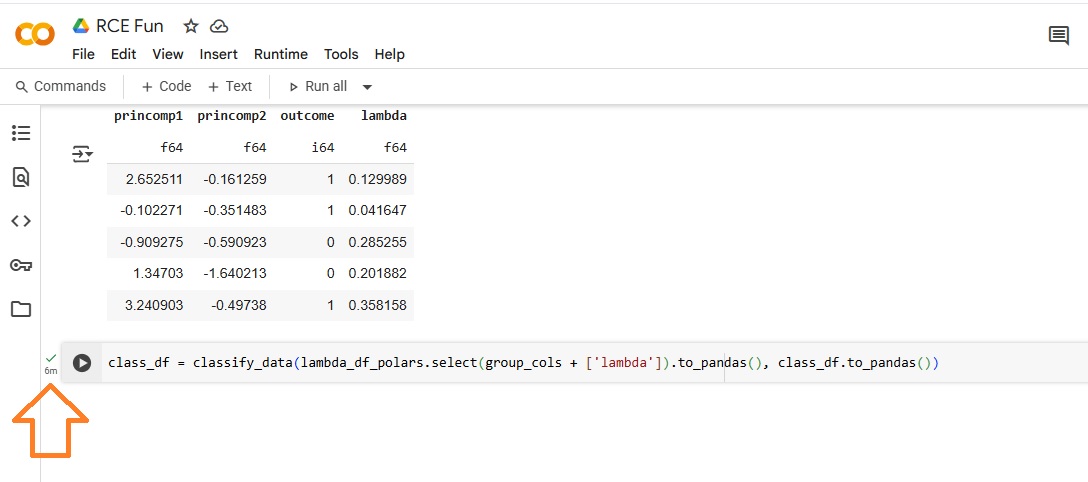
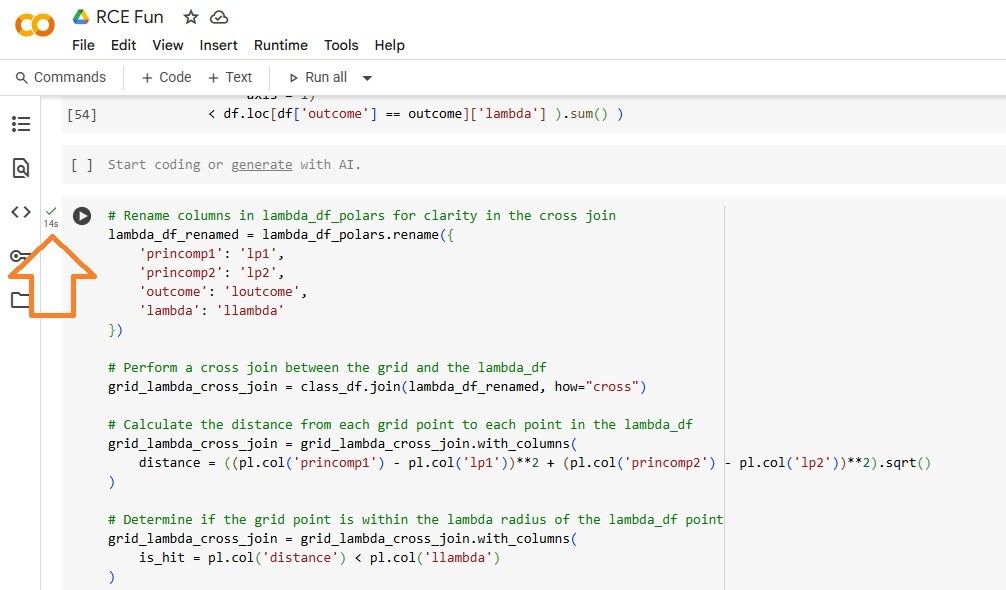
The wall clock time for the Polars approach reads fourteen (14) seconds, a ~25x improvement.
Data Viz
Last month, I created a graphic of the Pima Data set, which depicts the observations classified by Outcome 1 vs. Outcome 2.
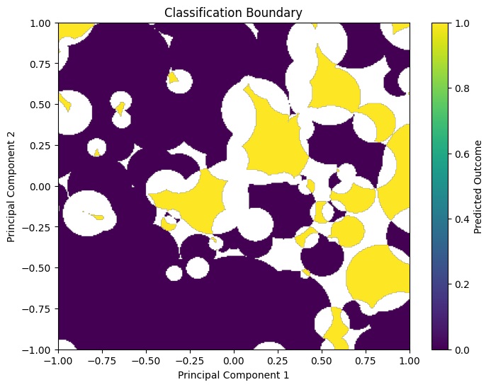
To graph it, I trained the Pima Dataset via RCE to generate a model. I then created a two-dimensional 300x300 grid DataFrame, and used the Pima model to classify all 9k points.
I will extend this to three dimensions. To do so, I must (1) reduce the Pima Dataset to 3D, (2) calculate the lambdas (radii) for all hit footprints, (3) create a 300x300x300 grid Data Viz (27,000,000 points) DataFrame, and (4) classify all 27M Data Viz points with the 3d model.
1. Reduce the Pima Data Set to Three Dimensions
The Pima Diabetes Dataset includes eight (8) features and one (1) target. For a 3D plot, I need to reduce the eight (8) features down to three (3). Principal Component Analysis (PCA) reduces dimensionality while retaining information. See my blog post New Exemplar Machine Learning Algorithm for a discussion on PCA. To laymen, PCA crams the observations from higher to lower-dimensional space. Imagine a bunch of coins sprinkled on a (2D) piece of paper. If you arrange them in a line, you just reduced the dimensionality. PCA executes the same process, but accounts for variance and density of the observations in the higher space.
First, I load the Pima Diabetes Dataset.
import numpy as np
import pandas as pd
import tensorflow as tf
import polars as pl

url = "https://raw.githubusercontent.com/plotly/datasets/master/diabetes.csv"
df_pima = pd.read_csv(url)
display(df_pima.head())

   Pregnancies  Glucose  BloodPressure  SkinThickness  Insulin   BMI  \
0            6      148             72             35        0  33.6
1            1       85             66             29        0  26.6
2            8      183             64              0        0  23.3
3            1       89             66             23       94  28.1
4            0      137             40             35      168  43.1

   DiabetesPedigreeFunction  Age  Outcome
0                     0.627   50        1
1                     0.351   31        0
2                     0.672   32        1
3                     0.167   21        0
4                     2.288   33        1
I create a Normalizer.
import tensorflow as tf
from tensorflow import keras
from tensorflow.keras import layers
from tensorflow.keras.layers import Normalization

pima_df = df_pima.copy()
labels = pima_df.pop('Outcome')

normalizer = Normalization()
normalizer.adapt(np
                 .array(pima_df))
I then run PCA on the normalized Pima Dataset. This collapses the eight (8) dimensions to three (3).
from sklearn.decomposition import PCA

pca = PCA(n_components=3)
pca.fit(normalizer(pima_df))
pca_features_df = pd.DataFrame(pca.transform(normalizer(pima_df)),
                                     columns = ['princomp1',
                                                'princomp2',
                                                'princomp3'],
                                     index=pima_df.index)

pima_df = pca_features_df.assign(outcome = labels)
This gives us the 3D Pima training dataset for RCE modeling.
print(pima_df.head())

   princomp1  princomp2  princomp3  outcome
0   1.068502   1.234895  -0.095930        1
1  -1.121683  -0.733852   0.712938        0
2  -0.396477   1.595876  -1.760679        1
3  -1.115781  -1.271241   0.663729        0
4   2.359335  -2.184819  -2.963107        1
2. Calculate the radii for all hit footprints
In RCE, lambdas (overloaded term) record the distance from an observation to the closest observation in a different class. RCE uses the lambdas to tally hits. We must calculate lambda for every observation in the training Dataset. I go into the code in my prior blog post. I also share the code at the bottom of this blog post. I wrote the code to accommodate an arbitrary number of dimensions.
Overload Warning: RCE uses lambda to indicate hit footprint radii. Pandas uses lambda to indicate inline/ anonymous functions. Do not confuse the two.
The following head() shows the observations with their target and lambda.
shape: (5, 5)
┌───────────┬───────────┬───────────┬─────────┬──────────┐
│ princomp1 ┆ princomp2 ┆ princomp3 ┆ outcome ┆ lambda   │
│ ---       ┆ ---       ┆ ---       ┆ ---     ┆ ---      │
│ f64       ┆ f64       ┆ f64       ┆ i64     ┆ f64      │
╞═══════════╪═══════════╪═══════════╪═════════╪══════════╡
│ -3.183769 ┆ -1.553631 ┆ 1.571653  ┆ 0       ┆ 2.399091 │
│ -1.038747 ┆ 1.269651  ┆ 0.878596  ┆ 1       ┆ 0.180943 │
│ -0.847973 ┆ 1.281973  ┆ -0.178098 ┆ 0       ┆ 0.209617 │
│ -0.546354 ┆ 1.100635  ┆ -0.542195 ┆ 1       ┆ 0.371084 │
│ -0.991178 ┆ -1.153642 ┆ -0.04556  ┆ 0       ┆ 0.587108 │
└───────────┴───────────┴───────────┴─────────┴──────────┘
3. Generate a 300x300x300 Data Viz Grid
The following code creates a Polars DataFrame with 27M Data Viz points. We will use this DataFrame to draw a 3D map of the Pima Dataset, classified by Outcome.
grid_size = 300
grid_range = 2
grid_start = -1

class_df = pl.DataFrame(
    {
        "princomp1": [
            grid_start + x * (grid_range / (grid_size - 1))
            for x in range(grid_size)
        ] * (grid_size * grid_size),
        "princomp2": [
            grid_start + y * (grid_range / (grid_size - 1))
            for y in range(grid_size) for _ in range(grid_size)
        ] * grid_size,
        "princomp3": [
            grid_start + z * (grid_range / (grid_size - 1))
            for z in range(grid_size) for _ in range(grid_size * grid_size)
        ]
    }
)
print(class_df)

shape: (27_000_000, 3)
┌───────────┬───────────┬───────────┐
│ princomp1 ┆ princomp2 ┆ princomp3 │
│ ---       ┆ ---       ┆ ---       │
│ f64       ┆ f64       ┆ f64       │
╞═══════════╪═══════════╪═══════════╡
│ -1.0      ┆ -1.0      ┆ -1.0      │
│ -0.993311 ┆ -1.0      ┆ -1.0      │
│ -0.986622 ┆ -1.0      ┆ -1.0      │
│ -0.979933 ┆ -1.0      ┆ -1.0      │
│ -0.973244 ┆ -1.0      ┆ -1.0      │
│ …         ┆ …         ┆ …         │
│ 0.973244  ┆ 1.0       ┆ 1.0       │
│ 0.979933  ┆ 1.0       ┆ 1.0       │
│ 0.986622  ┆ 1.0       ┆ 1.0       │
│ 0.993311  ┆ 1.0       ┆ 1.0       │
│ 1.0       ┆ 1.0       ┆ 1.0       │
└───────────┴───────────┴───────────┘
4. Classify all 27M Data Points
I already discussed the algorithm and implementation of RCE classification in my prior blog post. Please click through to read. The algo uses lambda to calculate hits in a given hit footprint and, based on the hits assigns a class.
I wrote the code to accommodate an arbitrary number of dimensions, so I run it now without edits.
When I attempt to run it in my Collab notebook, however, I get the following error:
ComputeError: cross joins would produce more rows than fits into 2^32; consider compiling with polars-big-idx feature, or set to 'streaming.'
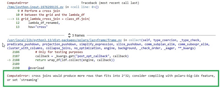
I want to use a cross join to leverage Polars/ Arrow distributed features. I could try to cobble together a different approach (manual chunking), but I don't have confidence in my ability to improve on the work done by the Polars developers. My hacked code would only bastardize the logic and execution of a cross join.
I instead use the Polars Streaming feature.
Quick aside. If I use the RCE epsilon hyperparameter and set an upper limit for the hit footprint size, this will greatly reduce the size of the model. I will show that in a future blog post. For now, I want to focus on illustrating the streaming feature of Polars.
Classification
I first set the Polars DataFrames to lazy.
lf_class  = class_df.lazy()
lf_lambda = lambda_df_polars.lazy()
I then load the RCE classification logic.
# Rename lambda-side cols
lf_lambda_renamed = lf_lambda.rename(
    {col: f"l{col}" for col in princomp_cols} | {"outcome": "loutcome", "lambda": "llambda"}
)

# Cross join (cartesian product)
lf_cross = lf_class.join(lf_lambda_renamed, how="cross")

# Distance calculation
distance_expr = (
    sum((pl.col(col) - pl.col(f"l{col}")) ** 2 for col in princomp_cols).sqrt()
)

lf_cross = lf_cross.with_columns(
    distance = distance_expr
)

# Flag hit
lf_cross = lf_cross.with_columns(
    is_hit = pl.col("distance") < pl.col("llambda")
)

# Group by the grid point
grid_group_cols = [col for col in class_df.columns if col.startswith("princomp")]

lf_hits = (
    lf_cross
    .group_by(grid_group_cols)
    .agg(
        ((pl.col("is_hit")) & (pl.col("loutcome") == 0)).sum().alias("hits_outcome_0"),
        ((pl.col("is_hit")) & (pl.col("loutcome") == 1)).sum().alias("hits_outcome_1"),
    )
    .with_columns(
        predicted_outcome = (
            pl.when( (pl.col("hits_outcome_0") > 0) & (pl.col("hits_outcome_1") == 0) )
              .then(0)
              .when( (pl.col("hits_outcome_1") > 0) & (pl.col("hits_outcome_0") == 0) )
              .then(1)
              .otherwise(None)     # unclassified
        )
    )
)
The pre-loaded logic processes the lazy input DataFrames into the lazy output DataFrame, which I name lf_hits (Lazy Fram Hits). I then execute the logic on the lf_hits, and set the Streaming flag.
hits_by_grid_point = lf_hits.collect(streaming=True)
After execution, we can take a peek at the DataFrame.
print(hits_by_grid_point.head())

┌───────────┬───────────┬───────────┬────────────────┬────────────────┬───────────────────┐
│ princomp1 ┆ princomp2 ┆ princomp3 ┆ hits_outcome_0 ┆ hits_outcome_1 ┆ predicted_outcome │
│ ---       ┆ ---       ┆ ---       ┆ ---            ┆ ---            ┆ ---               │
│ f64       ┆ f64       ┆ f64       ┆ u32            ┆ u32            ┆ i32               │
╞═══════════╪═══════════╪═══════════╪════════════════╪════════════════╪═══════════════════╡
│ 0.55102   ┆ -0.102041 ┆ -0.265306 ┆ 1              ┆ 2              ┆ null              │
│ -0.591837 ┆ -0.142857 ┆ 0.714286  ┆ 2              ┆ 0              ┆ 0                 │
│ 0.795918  ┆ 0.020408  ┆ -0.469388 ┆ 0              ┆ 0              ┆ null              │
│ 0.755102  ┆ -1.0      ┆ -0.020408 ┆ 1              ┆ 1              ┆ null              │
│ -0.632653 ┆ 0.510204  ┆ -1.0      ┆ 1              ┆ 1              ┆ null              │
└───────────┴───────────┴───────────┴────────────────┴────────────────┴───────────────────┘
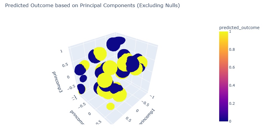
We can now plot the Classified Pima DataSet in 3D.
import plotly.express as px

filtered_hits_by_grid_point = hits_by_grid_point.filter(
    pl.col("predicted_outcome").is_not_null()
)

fig = px.scatter_3d(filtered_hits_by_grid_point.to_pandas(),
                    x='princomp1',
                    y='princomp2',
                    z='princomp3',
                    color='predicted_outcome',
                    title='Predicted Outcome based on Principal Components (Excluding Nulls)')
fig.show()
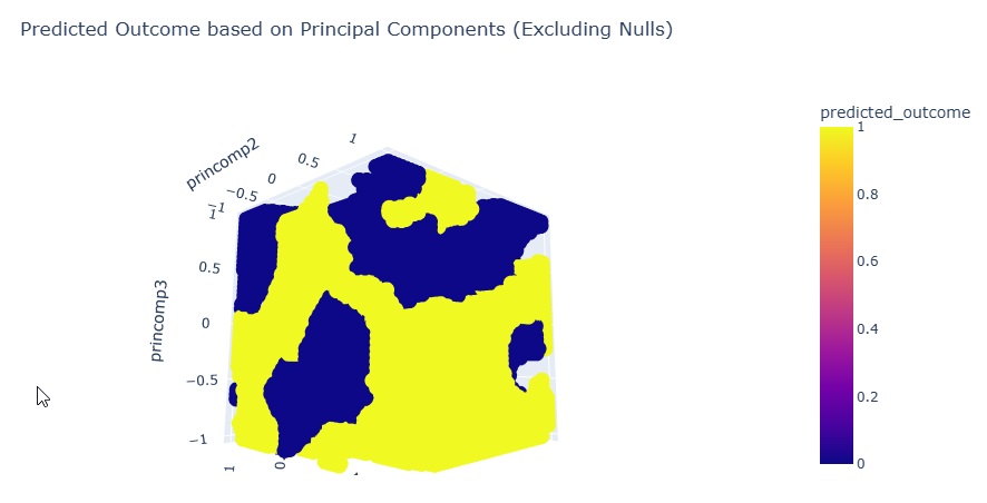
The plot shows Outcome 0 in yellow, and Outcome 1 in blue.
I tune the epsilon hyperparameter to put an upper limit on the hit footprints. This cleans up the plot.
Conclusion
Polars uses Apache Arrow to drive optimal utilization across every available core. For operations that clog local memory, like a cross join that yields a DataFrame larger than 32GB, Polars provides the Streaming construct. This sequentially loads chunks of data into memory, which drives parallel execution across time. Streaming allows Big Data computations on Collab notebooks and laptops. The Data Engineer does not need to concern herself with the housekeeping associated with most Big Data infrastructures. Remember the headaches that Hadoop and Spark caused? You do not need to deal with them; you just work with DataFrames and Polars figures the rest out.

Lambda Calculation Code
train_df_polars = pl.from_pandas(pima_df)

princomp_cols = [
    col for col in train_df_polars.columns if col.startswith('princomp')
]

join_selection = [
    pl.col(col).alias(f'{col}_other') for col in princomp_cols
] + [
    pl.col('outcome').alias('outcome_other')
]

df_with_other_outcome = train_df_polars.join(
    train_df_polars.select(
        princomp_cols + ['outcome']
    ).rename(
        {col: f'{col}_other' for col in princomp_cols} | {'outcome': 'outcome_other'}
    ),
    how="cross"
).filter(
    pl.col('outcome') != pl.col('outcome_other')
)

squared_distance_expr = sum(
    (pl.col(col) - pl.col(f'{col}_other'))**2 for col in princomp_cols
)

df_with_other_outcome = df_with_other_outcome.with_columns(
    squared_distance = squared_distance_expr
)

group_cols = [
    col for col in df_with_other_outcome.columns
    if col.startswith('princomp') and not col.endswith('_other')
] + ['outcome']

min_squared_dist_polars = (df_with_other_outcome
    .group_by(
        group_cols
    )
    .agg(
        pl.col("squared_distance")
        .min()
        .alias("min_squared_distance")
    )
)

lambda_df_polars = (min_squared_dist_polars
    .with_columns(
        pl.col("min_squared_distance")
        .sqrt()
        .alias("lambda")
    )
)

print(
    lambda_df_polars.select(
        group_cols + ['lambda']
    ).head()
)

┌───────────┬───────────┬───────────┬─────────┬──────────┐
│ princomp1 ┆ princomp2 ┆ princomp3 ┆ outcome ┆ lambda   │
│ ---       ┆ ---       ┆ ---       ┆ ---     ┆ ---      │
│ f64       ┆ f64       ┆ f64       ┆ i64     ┆ f64      │
╞═══════════╪═══════════╪═══════════╪═════════╪══════════╡
│ 0.466587  ┆ 0.42411   ┆ -0.133452 ┆ 0       ┆ 0.114694 │
│ -0.158603 ┆ 0.811361  ┆ 0.563424  ┆ 0       ┆ 0.430963 │
│ 0.395739  ┆ 1.375969  ┆ 0.234109  ┆ 0       ┆ 0.086674 │
│ -1.276773 ┆ -0.741043 ┆ -0.127401 ┆ 0       ┆ 0.546374 │
│ 0.91052   ┆ 1.058389  ┆ 0.605156  ┆ 1       ┆ 0.262343 │
└───────────┴───────────┴───────────┴─────────┴──────────┘