The open-source Polars library touts huge performance gains over Pandas. A combination of parallel processing, Apache Arrow, and a "Close to the Metal" Architecture drives Polars' speed. I refactored my Pandas-based Reduced Columb Energy (RCE) algorithm to Polars and will share my journey and observations with you.

The Reduced Columb Energy (RCE) Algorithm
The obscure RCE exemplar classifier offers a niche alternative to the well-known K-Nearest approach. I wrote about the algorithm in-depth in my New Exemplar Machine Learning Algorithm blog post.
The RCE algorithm labels inference data via hit footprints learned from training data.
RCE creates spheres around each labeled training observation, with radii equal to the distance of the closest labeled observation in the opposite class. The collection of all spheres for a given class represents the hit footprint for that class.
RCE uses the term lambda instead of the term radius. Lambda represents the radii of the spheres that comprise the hit footprints.
Look at the following diagram to understand the difference between RCE and K-Nearest.

In the diagram, we have two classes X and O. The green ? represents an observation in our inference data set. A training observation in class X sits closest to the green question mark.
K-Nearest would classify the green ? into class X since it sits closest to an observation in class X. RCE, however, classifies the Green ? into class O, because the unknown observation sits in the hit footprint of class O. The RCE hit footprint approach allows RCE to handle limited data sets.
Polars vs. Pandas
I need to overload terms in this discussion. The RCE algorithm uses the term lambda to represent radii. Pandas also uses the term lambda to represent inline/ anonymous functions. For clarity, I will use the term lambda when discussing the hit footprint radii, and lambda functions when discussing the Pandas anonymous functions. I hope that context will also drive clarity.
I take a functional approach to my Pandas development. I avoid iterative loops (for, while, if/then) and instead use the apply construct. I stuff data into a data frame, create a lambda function, and use the Pandas Data Frame apply method to process the data in a selection of columns via the lambda function. For you Map/ Reduce fans, the apply method covers the map side of the equation.
The Polars documentation, however, recommends that you avoid lambda functions:
Polars will try to parallelize the computation of the aggregating functions over the groups, so it is recommended that you avoid using lambdas and custom Python functions as much as possible. Instead, try to stay within the realm of the Polars expression API
Given this, I will use the native expression API vs. lambda functions when I refactor the code.

The Algorithm
I use the following approach to execute RCE in Pandas.
- Acquire Data and store in a Data Frame
- Split Data into Training and Inference Data Frames
- Apply a lambda function to each row (Observation) of the Training Set DataFrame and record the hit footprint for each Observation
- Apply a lambda function to each row in the Inference Set Dataframe and classify each Observation
Acquire Data and store in a Data Frame
The following code acquires our data and stores it in a data frame:
%pip install pandas_datareader

import numpy as np
import pandas as pd
import tensorflow as tf
import polars as pl

url = "https://raw.githubusercontent.com/plotly/datasets/master/diabetes.csv"
df_pima = pd.read_csv(url)
display(df_pima.head())
Split Data into Training and Inference Data Frames
We copy the data frame and execute a split.
pima_df = (df_pima
            .copy())

train_dataset = (pima_df
                  .sample(frac=0.8,
                               random_state = 0))

test_dataset = (pima_df
                .drop(train_dataset
                       .index))

train_features = (train_dataset
                  .copy())
test_features = (test_dataset
                  .copy())

train_labels = (train_features
                 .pop('Outcome'))
test_labels = (test_features
               .pop('Outcome'))
To help with plots, I use Principal Component Analysis (PCA) to reduce the dimensions of the training data.
from tensorflow import keras
from tensorflow.keras import layers
from tensorflow.keras.layers import Normalization

normalizer = Normalization()

normalizer.adapt(np
                 .array(train_features))


from sklearn.decomposition import PCA
pca = PCA(n_components=1)
pca.fit(normalizer(train_features))

pca_train_features_df = pd.DataFrame(pca.transform(normalizer(train_features)),
                                     columns = ['princomp1'],
                                     index=train_features.index)

pca = PCA(n_components=2)
pca.fit(normalizer(train_features))
pca_train_features_df = pd.DataFrame(pca.transform(normalizer(train_features)),
                                     columns = ['princomp1',
                                                'princomp2'],
                                     index=train_features.index)

train_df = pca_train_features_df.assign(outcome = train_labels)
If you would like to learn more about my justification and approach to dimensionality reduction, read my Pandas for RCE blog post.
Calculate Hit Footprints (Pandas)
In Pandas, I apply a lambda function to each row (Observation) of the Training Set Data Frame and record the hit footprint for each Observation.
RCE draws a circle around each labeled training observation, with a radius (lambda) that stops at the closest labeled training point in the opposite class. Each circle indicates the hit footprint for that class.
I use this code for the lambda function. Note that the function inputs the entire training data set. For each observation, I need to calculate the distance to every observation in the Train Dataframe (of a different class), and then select the closest.
def find_lambda(df, v):
  return ( np
            .linalg
            .norm(df
                    .loc[df['outcome'] != v[-1]]
                    .iloc[:,:-1]
                    .sub(np
                           .array(v[:-1])),
                  axis = 1)
            .min())
The lambda function executes the following for each observation:
- Remove all observations of the same class from the dataset
- Calculate the distance to every other observation in the filtered data set
- Choose the closest observation, and use the distance for lambda
TIP: Paste the above code into Collab and press the Explain button. Gemini will explain the code to you!
Classify Inference Data Frame (Pandas)
I create another lambda function to find the hits.
def find_hits(df, v, outcome ):
  return (( np
            .linalg
            .norm(df
                    .loc[df['outcome'] == outcome]
                    .iloc[:,:-2]
                    .sub(np
                           .array(v)),
                  axis = 1)
             < df.loc[df['outcome'] == outcome]['lambda'] ).sum() )
find_hits uses find_lambda, and I apply find_hits to the inference data frame to classify data.
def classify_data(training_df, class_df):
    # find the hits
    class0_hits = (class_df
                   .apply(lambda X: find_hits(training_df, X, 0),
                          axis = 1))
    class1_hits = (class_df
                   .apply(lambda X: find_hits(training_df, X, 1),
                          axis = 1))
    # add the columns
    class_df = (class_df
                .assign( class0_hits = class0_hits))
    class_df = (class_df
                .assign( class1_hits = class1_hits))
    # ID ambiguous, class 0 and class 1 data
    class_df['classification'] = np.nan
    class_df['classification'] = (class_df
                                  .apply(lambda X: 0 if X.class0_hits > 0 and X.class1_hits == 0 else X.classification,
                                         axis = 1))
    class_df['classification'] = (class_df
                                  .apply(lambda X: 1 if X.class1_hits > 0 and X.class0_hits == 0 else X.classification,
                                         axis = 1))
    return class_df
The Classification applies a lambda function to each row.
The algorithm only labels a class if one class registers at least one hit and the other classes register no hits. We can tune the algorithm to look at different weight options if desired.
Lambda vs. Expression API
The following diagram shows the current Pandas approach. I apply a lambda function to each row (Observation) in the Training Data Frame. Each call of the lambda function ingests a subset of the Training Data Frame that includes every observation of the opposite class. The original lambda function includes a nested lambda function that executes find_lambda, which uses the ingested Training Data Frame for each call.
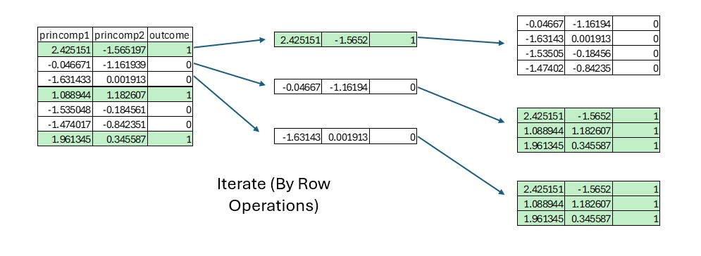
Every row of the Training Data Frame must calculate the distance to every other row in the Training Data Frame (of opposite class). We can either execute this logic via the application of lambda functions or via a cross join.
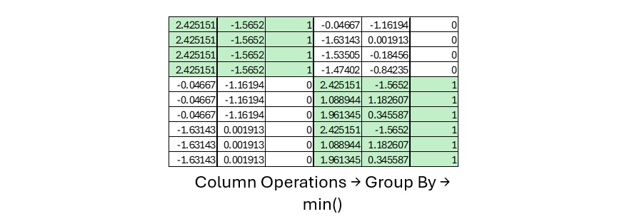
A cross join creates a Data Frame that includes every observation combined with every other observation (of opposite class). In this form, we can use Data Frame level operations to calculate distances. This allows Column Based processing vs. Row Based processing.
Once we have the distances in the cross join Data Frame, we can use a GROUP BY to find the min and therefore lambda (hit footprint radius) for each observation in the Training Dataframe.
Calculate Hit Footprints (Polars)
For Polars, we use the Polars expression API instead of lambda functions.
First, we:
- Get the list of principal component columns
- Create a selection for the cross join, and rename the Principal Component (princomp) columns in the right side Data Frame
- Cross-join the Data Frame with a subset of itself that includes opposite outcomes
NOTE: We include code (starts with) to accommodate an arbitrary number of principal components.
train_df_polars = pl.from_pandas(train_df)

princomp_cols = [
    col for col in train_df_polars.columns if col.startswith('princomp')
]

join_selection = [
    pl.col(col).alias(f'{col}_other') for col in princomp_cols
] + [
    pl.col('outcome').alias('outcome_other')
]

df_with_other_outcome = train_df_polars.join(
    train_df_polars.select(
        princomp_cols + ['outcome']
    ).rename(
        {col: f'{col}_other' for col in princomp_cols} | {'outcome': 'outcome_other'}
    ),
    how="cross"
).filter(
    pl.col('outcome') != pl.col('outcome_other')
)
This yields our cross join Data Frame.
print(df_with_other_outcome.head())

┌───────────┬───────────┬─────────┬─────────────────┬─────────────────┬───────────────┐
│ princomp1 ┆ princomp2 ┆ outcome ┆ princomp1_other ┆ princomp2_other ┆ outcome_other │
│ ---       ┆ ---       ┆ ---     ┆ ---             ┆ ---             ┆ ---           │
│ f64       ┆ f64       ┆ i64     ┆ f64             ┆ f64             ┆ i64           │
╞═══════════╪═══════════╪═════════╪═════════════════╪═════════════════╪═══════════════╡
│ 2.425151  ┆ -1.565197 ┆ 1       ┆ -0.046671       ┆ -1.161939       ┆ 0             │
│ 2.425151  ┆ -1.565197 ┆ 1       ┆ -1.631433       ┆ 0.001913        ┆ 0             │
│ 2.425151  ┆ -1.565197 ┆ 1       ┆ -1.535048       ┆ -0.184561       ┆ 0             │
│ 2.425151  ┆ -1.565197 ┆ 1       ┆ -1.474017       ┆ -0.842351       ┆ 0             │
│ 2.425151  ┆ -1.565197 ┆ 1       ┆ 1.105778        ┆ -1.756428       ┆ 0             │
└───────────┴───────────┴─────────┴─────────────────┴─────────────────┴───────────────┘
To find the distances to every other point of the opposite class, we execute:
squared_distance_expr = sum(
    (pl.col(col) - pl.col(f'{col}_other'))**2 for col in princomp_cols
)

df_with_other_outcome = df_with_other_outcome.with_columns(
    squared_distance = squared_distance_expr
)
Notice the column based operations, which use -, + and ** (square) on the columns princomp1 and princomp2. The operations yield the squared distance for the cross-joined Data Frame.
print(df_with_other_outcome.head())

┌───────────┬───────────┬─────────┬────────────────┬───────────────┬───────────────┬───────────────┐
│ princomp1 ┆ princomp2 ┆ outcome ┆ princomp1_othe ┆ princomp2_oth ┆ outcome_other ┆ squared_dista │
│ ---       ┆ ---       ┆ ---     ┆ r              ┆ er            ┆ ---           ┆ nce           │
│ f64       ┆ f64       ┆ i64     ┆ ---            ┆ ---           ┆ i64           ┆ ---           │
│           ┆           ┆         ┆ f64            ┆ f64           ┆               ┆ f64           │
╞═══════════╪═══════════╪═════════╪════════════════╪═══════════════╪═══════════════╪═══════════════╡
│ 2.425151  ┆ -1.565197 ┆ 1       ┆ -0.046671      ┆ -1.161939     ┆ 0             ┆ 6.272523      │
│ 2.425151  ┆ -1.565197 ┆ 1       ┆ -1.631433      ┆ 0.001913      ┆ 0             ┆ 18.911708     │
│ 2.425151  ┆ -1.565197 ┆ 1       ┆ -1.535048      ┆ -0.184561     ┆ 0             ┆ 17.589336     │
│ 2.425151  ┆ -1.565197 ┆ 1       ┆ -1.474017      ┆ -0.842351     ┆ 0             ┆ 15.726017     │
│ 2.425151  ┆ -1.565197 ┆ 1       ┆ 1.105778       ┆ -1.756428     ┆ 0             ┆ 1.777314      │
└───────────┴───────────┴─────────┴────────────────┴───────────────┴───────────────┴───────────────┘
A GROUP BY followed by the min operation returns the minimum squared distance for each operation.
group_cols = [
    col for col in df_with_other_outcome.columns
    if col.startswith('princomp') and not col.endswith('_other')
] + ['outcome']

min_squared_dist_polars = (df_with_other_outcome
    .group_by(
        group_cols
    )
    .agg(
        pl.col("squared_distance")
        .min()
        .alias("min_squared_distance")
    )
)
The square root operation gives us the minimum Euclidean distance, or lambda.
lambda_df_polars = (min_squared_dist_polars
    .with_columns(
        pl.col("min_squared_distance")
        .sqrt()
        .alias("lambda")
    )
)
We now have a Training Data Frame that records every lambda (hit footprint radius) for every Observation.
print(
    lambda_df_polars.select(
        group_cols + ['lambda']
    ).head()
)

┌───────────┬───────────┬─────────┬──────────┐
│ princomp1 ┆ princomp2 ┆ outcome ┆ lambda   │
│ ---       ┆ ---       ┆ ---     ┆ ---      │
│ f64       ┆ f64       ┆ i64     ┆ f64      │
╞═══════════╪═══════════╪═════════╪══════════╡
│ -0.242788 ┆ -1.433054 ┆ 1       ┆ 0.030056 │
│ -1.035114 ┆ -0.063441 ┆ 0       ┆ 0.087633 │
│ 0.237591  ┆ 1.848636  ┆ 1       ┆ 0.130412 │
│ 0.477868  ┆ 1.650595  ┆ 0       ┆ 0.123065 │
│ 1.136271  ┆ -1.039659 ┆ 0       ┆ 0.140668 │
└───────────┴───────────┴─────────┴──────────┘
Classify Inference Data Frame (Polars)
We refactor our algorithm to use the Polars expression API instead of lambda functions.
First, we create a 2D grid of data. The grid provides the Inference Dataframe. This code assumes we have only two Principal Components.
grid_size = 300
grid_range = 2
grid_start = -1

class_df \
    = pl.DataFrame(
        {
            "princomp1": [
                grid_start
                + x
                * (
                    grid_range
                    / (
                        grid_size
                        - 1
                    )
                ) for x in range(grid_size)
            ]
            * grid_size,
            "princomp2": [
                grid_start
                + y
                * (
                    grid_range
                    / (
                        grid_size
                        - 1
                    )
                ) for y in range(grid_size) for _ in range(grid_size)
            ]
        }
    )
The Polars classification approach
- Cross joins the Inference Data Frame and the Training Data Frame to drive Column Based, Group By and Summary Statistic (Sum) operations
- Calculates the Euclidean distance between each Observation in the Inference Data Frame and each point in the Training Data Frame
- Identifies Hits, when the Euclidean distance clocks in less than the lambda (footprint radius) distance
- Aggregates the hits. For now, we only classify a hit if an observation lies in only one class (we can tune this)
# Cross join
lambda_df_renamed = lambda_df_polars.rename(
    {
        col: f'l{col}' for col in princomp_cols
    } | {'outcome': 'loutcome', 'lambda': 'llambda'}
)

grid_lambda_cross_join = class_df.join(
    lambda_df_renamed,
    how="cross"
)

# Find Euclidean Distances
distance_expr = sum(
    (pl.col(col) - pl.col(f'l{col}'))**2 for col in princomp_cols
).sqrt()

grid_lambda_cross_join = (grid_lambda_cross_join
    .with_columns(
        distance = distance_expr
    )
)

# ID Hits
grid_lambda_cross_join = (grid_lambda_cross_join
    .with_columns(
        is_hit = pl.col('distance') < pl.col('llambda')
    )
)

# GROUP BY and SUM hits
grid_group_cols = [col for col in class_df.columns if col.startswith('princomp')]
hits_by_grid_point = (grid_lambda_cross_join
    .group_by(grid_group_cols)
    .agg(
        (pl.col('is_hit') & (pl.col('loutcome') == 0))
        .sum()
        .alias('hits_outcome_0'),
        (pl.col('is_hit') & (pl.col('loutcome') == 1))
        .sum()
        .alias('hits_outcome_1')
    )
)

# Decide on class
hits_by_grid_point = (hits_by_grid_point
    .with_columns(
        predicted_outcome = pl.when(
                                (pl.col('hits_outcome_0') > 0) &
                                (pl.col('hits_outcome_1') == 0)
                            )
                            .then(0)
                            .when(
                                (pl.col('hits_outcome_1') > 0) &
                                (pl.col('hits_outcome_0') == 0)
                            )
                            .then(1)
                            .otherwise(None)
    )
)
This yields a classified Inference Data Frame:
print(hits_by_grid_point.head())

┌───────────┬───────────┬────────────────┬────────────────┬───────────────────┐
│ princomp1 ┆ princomp2 ┆ hits_outcome_0 ┆ hits_outcome_1 ┆ predicted_outcome │
│ ---       ┆ ---       ┆ ---            ┆ ---            ┆ ---               │
│ f64       ┆ f64       ┆ u32            ┆ u32            ┆ i32               │
╞═══════════╪═══════════╪════════════════╪════════════════╪═══════════════════╡
│ 0.913043  ┆ -0.498328 ┆ 0              ┆ 1              ┆ 1                 │
│ 0.591973  ┆ 0.498328  ┆ 0              ┆ 1              ┆ 1                 │
│ -0.277592 ┆ -0.110368 ┆ 0              ┆ 2              ┆ 1                 │
│ -0.531773 ┆ 0.571906  ┆ 4              ┆ 0              ┆ 0                 │
│ -0.478261 ┆ -0.973244 ┆ 11             ┆ 0              ┆ 0                 │
└───────────┴───────────┴────────────────┴────────────────┴───────────────────┘
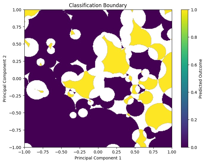
We plot a heat map of the Classified Data:
import matplotlib.pyplot as plt
import numpy as np

# Polars to Pandas for Matplotlib
hits_by_grid_point_pd = hits_by_grid_point.to_pandas()

# Pivot and sort data for Heatmap
hits_by_grid_point_pd = hits_by_grid_point_pd.sort_values(
    by=['princomp2', 'princomp1']
)

# Reshape to 300x300 grid
grid_size = 300 # Update grid_size to match the actual grid size
predicted_outcome_grid = hits_by_grid_point_pd[
    'predicted_outcome'
].values.reshape(
    (grid_size, grid_size)
)

# Set Axis
princomp1_values = hits_by_grid_point_pd['princomp1'].unique()
princomp2_values = hits_by_grid_point_pd['princomp2'].unique()

# Heatmap
plt.figure(figsize=(8, 6))
plt.imshow(
    predicted_outcome_grid,
    origin='lower',
    extent=[
        princomp1_values.min(),
        princomp1_values.max(),
        princomp2_values.min(),
        princomp2_values.max()
    ],
    aspect='auto',
    cmap='viridis'
)
plt.colorbar(label='Predicted Outcome')
plt.title('Classification Boundary')
plt.xlabel('Principal Component 1')
plt.ylabel('Principal Component 2')
plt.show()
Execution Time
I used the same Python environment to run my algorithm on the same data set in both Pandas and Polars. I saw a significant reduction in wall clock time to complete the processing.
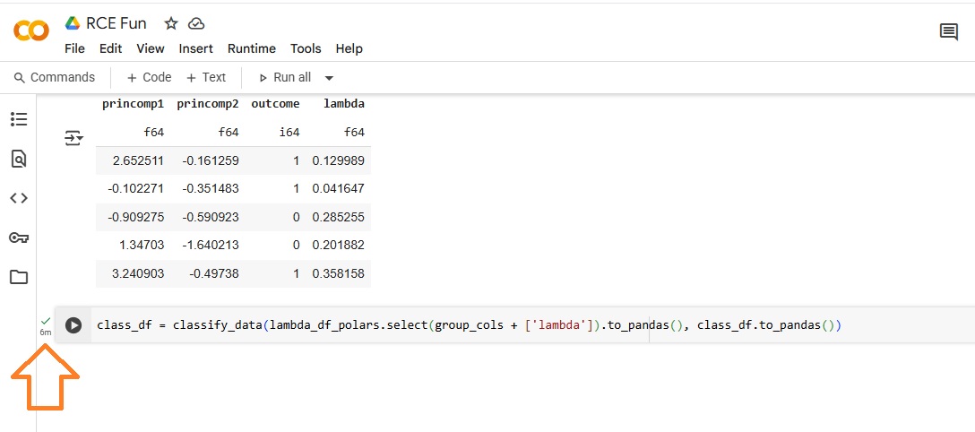
The Pandas (lambda) approach took roughly six (6) minutes to complete.
The Polars approach took only fourteen (14)seconds, a reduction of 96%.
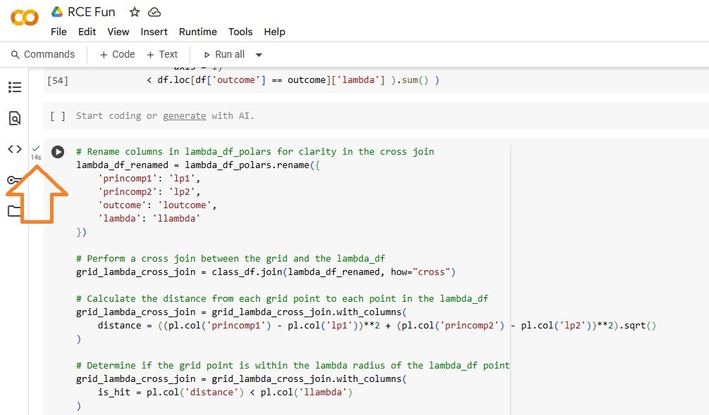
This reduction of 96% equates to a performance gain of 25x.
Conclusion
The cross-join approach, in addition to the parallel architecture of Polars, yielded a 25x boost over Pandas. The crossr-join, however, requires the compute to hold n2 rows and 2m columns in memory, given n rows in the training set with m feature columns. Next month I will look at a way to mitigate the scenario where the cross-join Data Frame exceeds available memory.