Sealed and Graded Video Game Collecting skyrocketed in popularity over the past decade. I joined the hobby in 2020 and stuck through the boom times of 2021 and the recent crash of 2023.
Background
Despite the recent crash, sealed video games do provide organic collectability. In contrast to Image Comics (Gold Editions! Holo-Foil Covers!) and Star Wars Power of the Force (Green Cardboard! Brown Vest Luke!) action figures, no one (that I knew of) thought to preserve outdated, legacy video games in the 1990s.
In 1993, for example, I traded about $10 worth of (completely legal) fireworks for the 8-Bit Nintendo Entertainment System (NES) releases of Wrestlemania, Mega Man, and (IIRC) Jackal.
Nobody (except a handful of weirdos) kept sealed copies of NES, Genesis, or SNES games. If I got a game, I opened it and played it, end of story. Today, the supply of conventional collectibles (comics, sports cards, action figures) dwarfs the supply of sealed video games.
On the demand side, sealed Video games, like the NFT market, appear to follow a winner take all approach. The popular, or brand name games sell at multiples of less popular games, with no regard for supply. You can, for example, buy certain pop one (only one known sealed game in the market) games on Heritage for a little under $200 at auction.
DISCLAIMER: I base the information on this blog on my personal opinion and experience and you MUST not consider this professional financial investment advice. Do not ever use my opinions without first assessing your own personal and financial and situation and you MUST consult a financial professional before making any investment. Keep in mind I will change my thoughts and opinions over time as I learn and accumulate more knowledge. I am NOT a financial professional! This blog is not a place for the giving or receiving financial advice, advice concerning investment decisions or tax or legal advice.
Investment Grade
Today we analyze the collectability of Super Mario Bros. 3 for the NES.
Shawn Surmick from Reserved Investments taught me the idea of an Investment Grade collectible, a collectible in the 85th percentile of the population.
Investment-grade collectibles sit at the top 15% of the pack.
The CGC census, for example, records 623 graded copies of the 1962 issue of Green Lantern #16 (First Star Sapphire). 623 times 15% yields the quantity 93.45. If you add the quantities for each universal grade, you will find that less than 94 copies of this comic have a grade of greater than 8.5. For that reason, an investor can consider any copy of Green Lantern #16 (1962) with a grade equal to or greater than 8.5 Investment Grade.
A glance at the census for Super Mario 3, however, indicates a need for a more complicated analysis.
Import and Clean the Data
We use the Python Pandas package for our analysis, and Python Seaborn fuels the graphics.
We use data from Larry's GamerStonks (non-affiliate link) database.
If you want to collect sealed video games, then I recommend you pay for a subscription to Gamerstonks.
We load the libraries and import the data from a Comma Separated Value (CSV) spreadsheet into a Pandas DataFrame.
import pandas as pd
import numpy as np
import seaborn as sns
import matplotlib.pyplot as plt

sns.set(rc={'figure.figsize':(11.7,8.27)})

df = pd.read_csv('smb3.csv')
The DataFrame includes the Grader (WATA, CGC), Box Grade, Seal Grade, Variant, Purchase Price, Auction House (Goldin, Heritage, Certified Link), and the Date Sold.
Grader Box Seal Variant                                            Price  Auction           Date
WATA   9.6 A    *Made in Japan, Oval SOQ R - "USA, Canada and ...  $2,880 Heritage Auctions 11/30/23
WATA   9.4 A    *Made in Japan, Oval SOQ R - "USA, Canada and ...  $2,160 Heritage Auctions 11/30/23
WATA   8.0 A    *Made in Japan, Oval SOQ R - "USA, Canada and ...  $1,159 Goldin            11/18/23
WATA   9.6 A+   *Made in Japan, NFR (Challenge Set)                $2,160 Heritage Auctions 11/04/23
...
We need to encode the data into the correct type, for example, convert Price from String to Numeric, and Date from String to DateTime.
df['Date'] = pd.to_datetime(df['Date'])
df['Price'] = df['Price'].str.replace('$', '').str.replace(',', '').astype(float)
The Seal ratings, while of type String, represent a scale of increasing preference. We use Pandas to encode Seal into an Ordered Categorical type.
df['Seal'] = pd.Categorical(df['Seal'], categories=['NS','C+','B+','A','A+','A++'], ordered=True)
Python indicates the hierarchy:
Categories (6, object):
['NS' < 'C+' < 'B+' < 'A' < 'A+' < 'A++']
Can we Use Box Grade for our Analysis?
CGC Comics provides a numeric score for quality. CGC and WATA video games both provide a numeric score for Box quality and also provide a Seal grade.
In the Green Lantern example above, we use the CGC Universal Grade to stack rank the comics and identify the investment grade. Can we use the WATA (or CGC) Sealed Video Game Box Grade to identify the investment grade for Super Mario 3 (SMB3)?
Consider the summary statistics for the Price of the 9.6 Box grade:
df[df['Box'] == 9.6]['Price'].describe()
Python dumps a ton of data.
count       28.000000
mean     11526.428571
std       8659.504825
min       2160.000000
25%       5220.000000
50%       8400.000000
75%      16350.000000
max      33600.000000
Name: Price, dtype: float64
For the twenty-eight (28) copies of SMB3 graded 9.6, we see a high sale price of $33.60k, a low of $2.16k, a median of $8.4k, and so on.
I now present to you a Box Plot.
sns.boxplot(x='Box', y='Price', data = df[df['Box'] == 9.6])
The Box Plot captures the information from the table in graphical form.
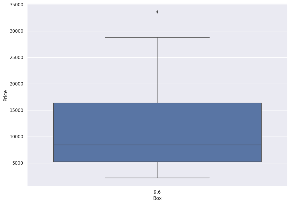
The box shows the First ($5.2k) and Third ($16.35k) quartiles and the whiskers show data points that lie 1.5 times the Interquartile range (IQR) (for both top and bottom). The little diamond shows the outliers, in this case, the max of $33.6k.
We plot the distribution for each of the recorded Box Grades:
sns.boxplot(x='Box', y='Price', data=df)
plt.axhline(df[df['Box'] == 9.8]['Price'].min(), color='red')
This yields:
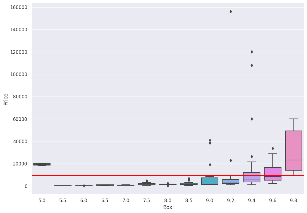
The red horizontal line captures the lowest price paid for a 9.8 Box grade.
The graph illustrates that certain instances of Box grades with scores of 9.6, 9.4, 9.2, 9.0, and even 5.0 (!) sold for more than the minimum 9.8 price.
A quick calculation illustrates that 23% of all copies graded less than 9.8 sold for more than the 9.8 minimum.
sum(df[df['Box'] < 9.8]['Price'] > df[df['Box'] == 9.8]['Price'].min())/df[df['Box'] < 9.8].shape[0]

0.23076923076923078
Based on this discovery, we can not use Box grade alone to identify the top 15% of SMB3.
Data Enrichment
InfluxDB uses the terms Tags and Measurements for Categorical and Continuous variables. Tags allow extra dimensions in Data Visualization.
We first create Tags for Year and Quarter. These provide buckets for aggregations.
df['Year'] = df['Date'].dt.year
df['Quarter'] = pd.PeriodIndex(df['Date'], freq='Q').strftime('%Y-0%q')
We also want to improve the readability of the Variant feature.
The Original Data Set uses WATA and CGC notes for the Variant column:
- *Made in Japan, NFR (Challenge Set)
- *Made in Japan, Oval SOQ R - "USA and Canada" Text
- *Made in Japan, Oval SOQ R - "USA, Canada and Mexico" Text
- *Made in Japan, Oval SOQ R - ""USA and Canada"" Text
- *Made in Japan, Oval SOQ TM - Left Bros.
- *Made in Japan, Oval SOQ TM - Right Bros.
- *Made in Japan, Oval SOQ R - ""USA, Canada and Mexico"" Text
To simplify the analysis, we shorten these variants to:
- NFR
- CAN
- MEX
- LEFT
- RIGHT
We create a quick lookup DataFrame and merge it into my working DataFrame.
tag_df = pd.DataFrame.from_dict({'Variant': ['*Made in Japan, Oval SOQ R - "USA, Canada and Mexico" Text',
  '*Made in Japan, NFR (Challenge Set)',
  '*Made in Japan, Oval SOQ R - "USA and Canada" Text',
  '*Made in Japan, Oval SOQ TM - Left Bros.',
  '*Made in Japan, Oval SOQ TM - Right Bros.',
  '*Made in Japan, Oval SOQ R - ""USA, Canada and Mexico"" Text',
  '*Made in Japan, Oval SOQ R - ""USA and Canada"" Text'],
  'Var_Tag': ['MEX','NFR','CAN','LEFT','RIGHT','MEX','CAN']
  })

 df = df.merge(tag_df, on='Variant', how='left')
This results in:
Grader Box Seal Variant                                           Price  Auction           Date       Year Quarter Var_Tag
WATA   9.6 A    *Made in Japan, Oval SOQ R - "USA, Canada and ... 2880.0 Heritage Auctions 2023-11-30 2023 2023-04 MEX
WATA   9.4 A    *Made in Japan, Oval SOQ R - "USA, Canada and ... 2160.0 Heritage Auctions 2023-11-30 2023 2023-04 MEX
WATA   8.0 A    *Made in Japan, Oval SOQ R - "USA, Canada and ... 1159.0 Goldin            2023-11-18 2023 2023-04 MEX
WATA   9.6 A+   *Made in Japan, NFR (Challenge Set)               2160.0 Heritage Auctions 2023-11-04 2023 2023-04 NFR
I dump the noisy and unused Columns:
df = df.dropna().drop(['Grader','Variant','Auction'], axis=1)
I synthesize a Categorical Price_Tag from the Numerical Price column. This allows us to visualize prices in four buckets: Lowest, Low, High and Highest.
df['Price_Tag'] = pd.qcut(df['Price'],q=4,labels=['Lowest','Low','High','Highest'])
The new Price_Tag feature allows quick and easy 3d plots.
sns.displot(df, x='Box',y='Seal',hue='Price_Tag')
Displot shows a heat map between the Box grade, the Seal grade and the Price.
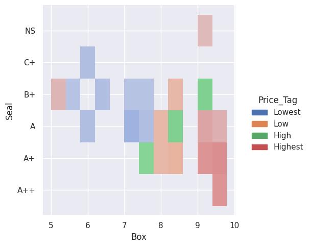
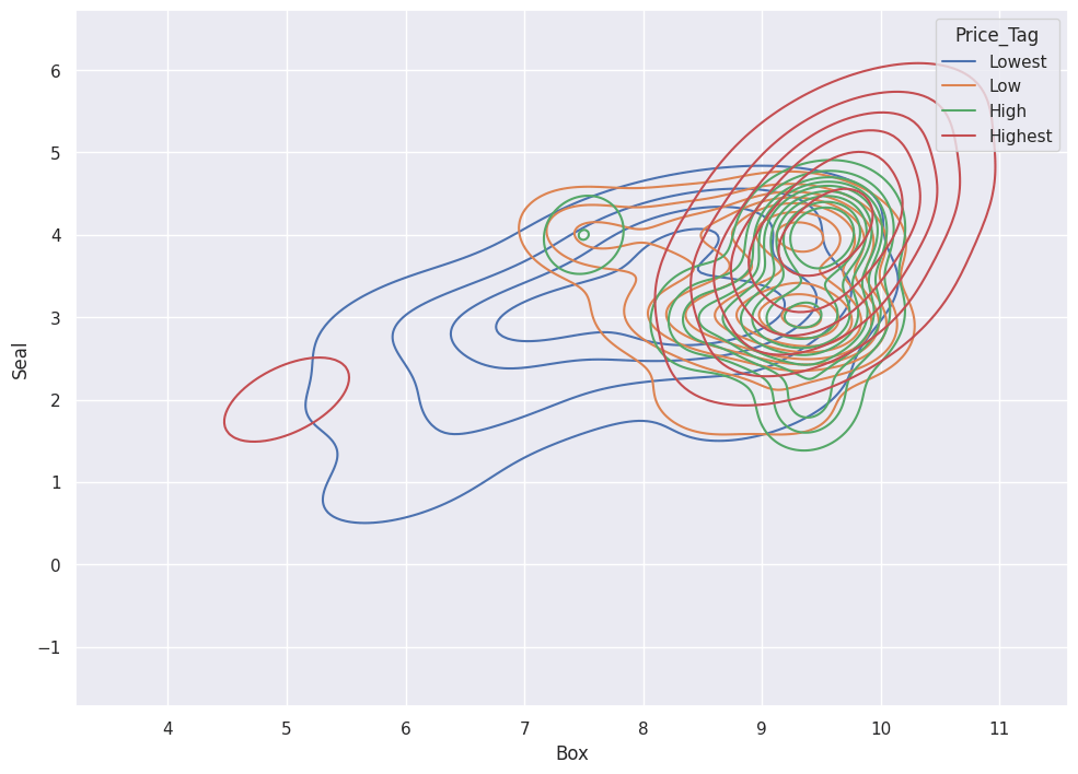
High Box grades cluster around A+ Seal grades, and low Box grades cluster around the B+ Seal grade. Price (Highest = Red) correlates with high Box and Seal Grades.
If you notice, the price for an 8.5 Box with an A Seal registers higher than the price for an 8.5 Box with an A+ Seal (Green vs. Orange).
Date and Variation's Effect on Price
The sealed, graded Video Game collectible market spiked and crashed since 2021.
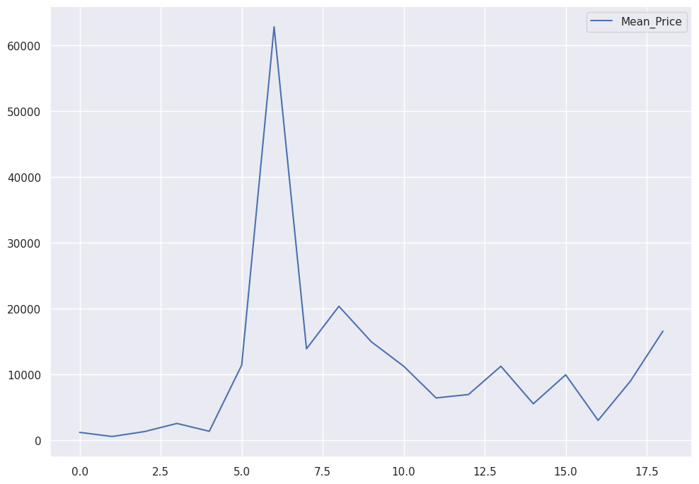
sns.lineplot(x='Year', y='Price', data=df)
The next chart shows the mean price over the years, with error bands that depict variation.
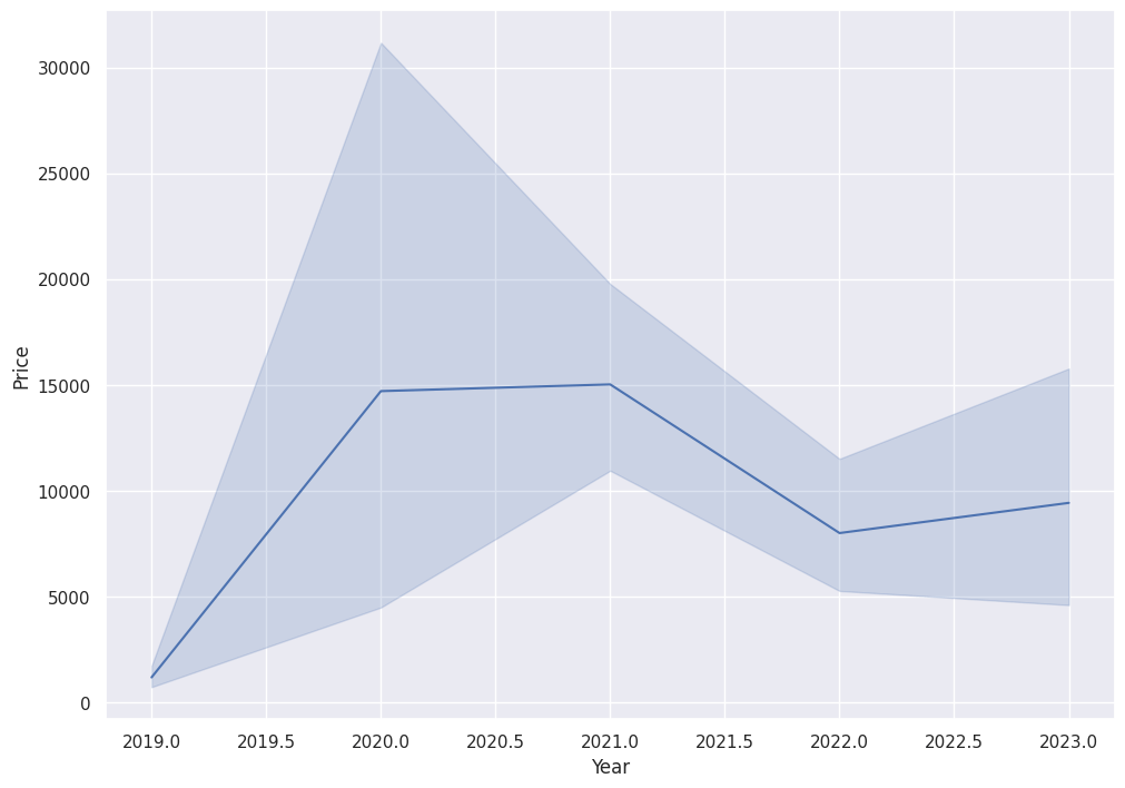
We see a peak in 2021.
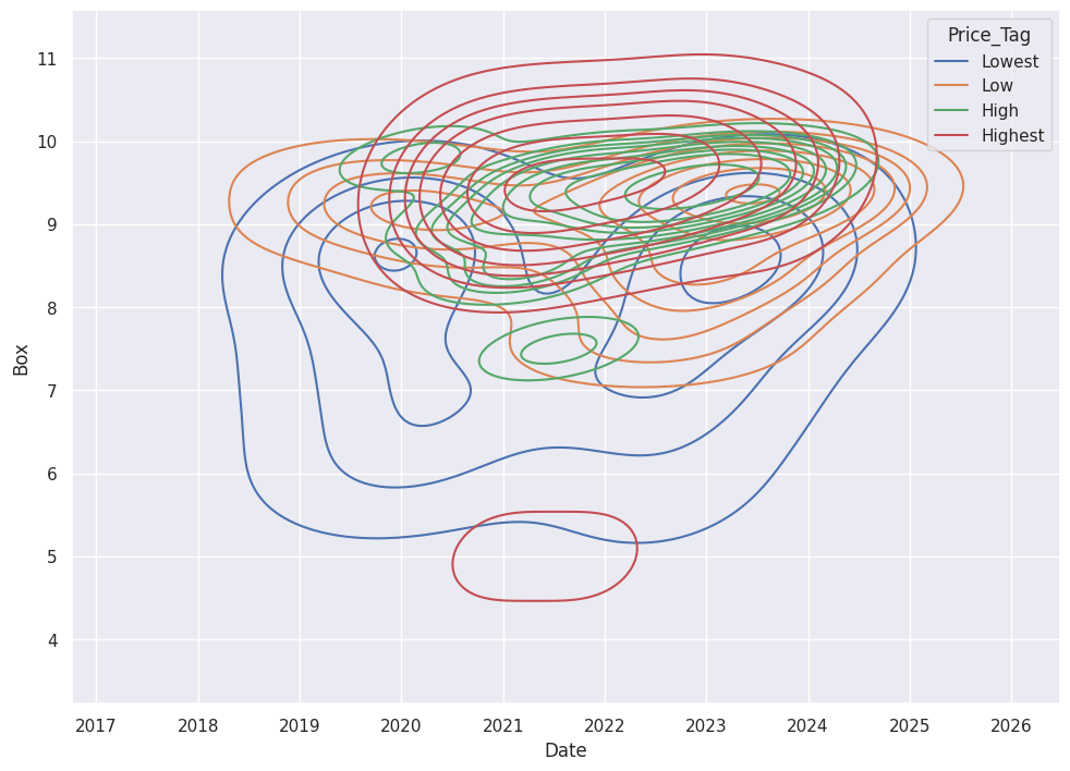
Look at the sales data in terms of Box Grade and Date Sold:
sns.kdeplot(df,x="Date",y='Box', hue='Price_Tag')
The highest sales cluster around the high Box Grades and 2021.
Variant drives Price along with the purchase Date.
sns.lineplot(x='Year', y='Price',hue='Var_Tag', data=df)
plt.ylim([0,df['Price'].quantile(q=0.99)])
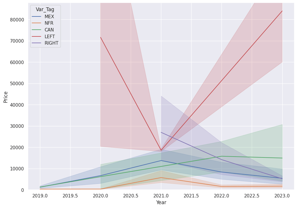
If we eyeball the chart, we see that the Left Bros. Variant trumps the Canada (No Mexico) Variant, which trumps Right Bros. and then Mexico variants. NFR sits at the bottom (which makes sense, because the seal contains the text Not for Resale which obfuscates the box art).
We will rank the Variant feature, therefore, in this order: NFR < MEX < RIGHT < CAN < LEFT
df['Var_Tag'] = pd.Categorical(df['Var_Tag'], categories=['NFR','MEX','RIGHT','CAN','LEFT'], ordered=True)
We use this new Categorical ranking to plot Box Grade vs. Sale Price vs. Var_Tag.
sns.boxplot(x='Box', y='Price',hue='Var_Tag', data=df[df['Box'] > 9.0])
This yields:
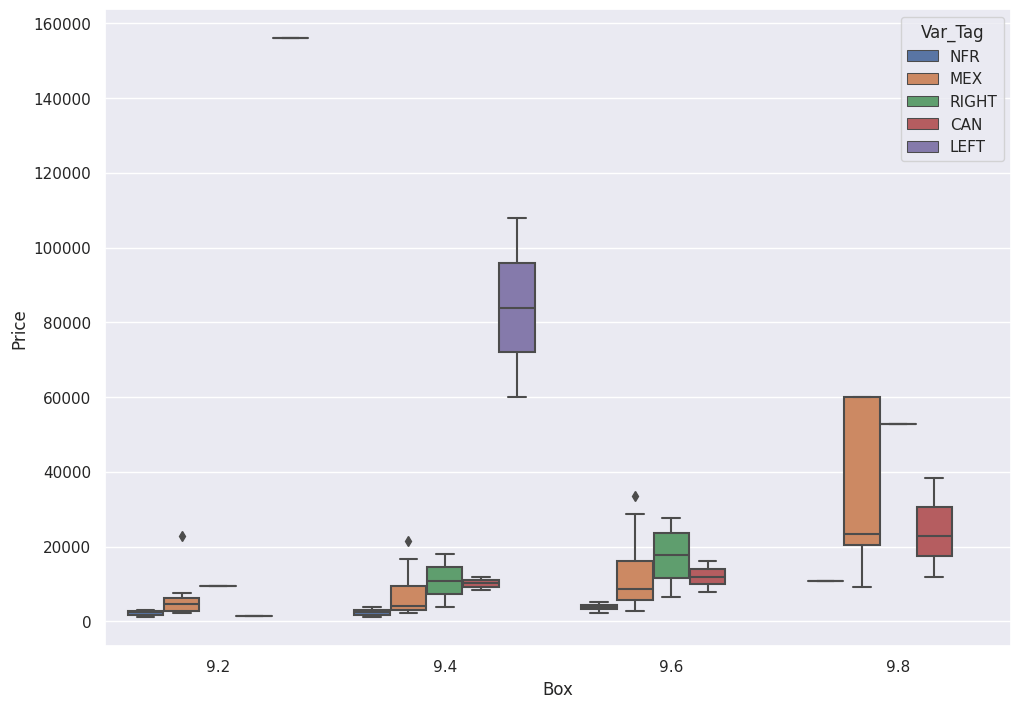
Note that the (Purple) LEFT Bros. variant trounces all the higher-graded variants.
We need to pay attention to Date and Variant.
Quick Aside: Numerical analysis
Pandas provides tools to convert Tags to Measurements ( Categorical to Numeric). Machine Learning, for example, requires normalized numeric data.
We create a numeric version of our DataFrame:
df_num = df.copy()
df_num['Seal'] = pd.factorize(df['Seal'],sort=True)[0]
df_num['Var_Tag'] = pd.factorize(df['Var_Tag'],sort=True)[0]
I input this numeric DataFrame into a Correlation Graphing Function to produce a Heat Map:
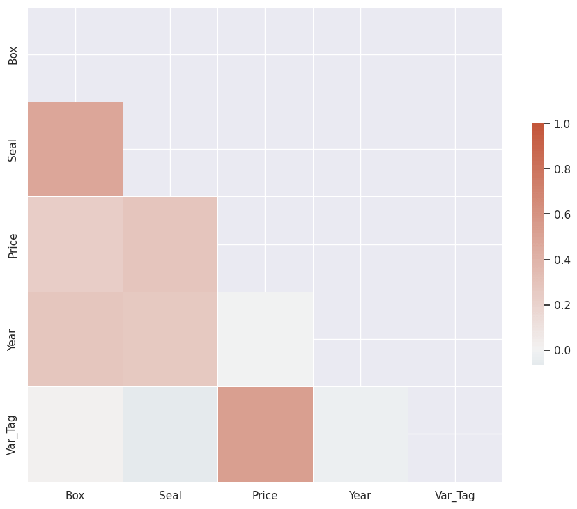
A Numeric encoding of Seal (NS, C+, B+, A, A++) allows us to use a Kernel Density Estimation plot for Box vs. Seal vs. Price.
sns.kdeplot(df_num,x="Box",y='Seal', hue='Price_Tag')
Normalize Price Over Time
Price lets us stack rank the different Variants and Box Grades of Super Mario Bros. 3.
The Sale Date variable also impacts the Sale Price.
We will remove (or at least mitigate) the effect of Sale Date on our price data.
We can choose from dozens of approaches. I choose the following approach to remove the impact of Date on the Price data:
- Calculate the Mean_Price per Quarter
- Normalize each Sale Price by its Quarter's Mean_Price
I first calculate the Mean_Price per Quarter:
af = df.set_index('Date').groupby('Quarter')['Price'].resample('A').mean().reset_index()
af.rename(columns={'Price': 'Mean_Price'}, inplace=True)
af.dropna(inplace=True)
af.drop(['Date'], axis=1, inplace=True)


    Quarter Mean_Price
0   2019-02 1176.000000
1   2019-03 552.000000
2   2019-04 1298.571429
3   2020-01 2534.400000
4   2020-02 1346.250000
5   2020-03 11397.333333
6   2020-04 62800.000000
7   2021-01 13878.750000
8   2021-02 20340.000000
9   2021-03 14948.571429
10  2021-04 11228.571429
11  2022-01 6408.333333
12  2022-02 6932.000000
13  2022-03 11226.800000
14  2022-04 5524.090909
15  2023-01 9927.428571
16  2023-02 3001.333333
17  2023-03 8980.000000
18  2023-04 16562.375000
We merge this lookup table with the working DataFrame.
df = df.merge(af, on=['Quarter'], how='left')
Create a feature Norm_Price which records the sale Price in units of Mean_Price.
df['Norm_Price'] = df['Price']/df['Mean_Price']
Calculate the normalized (against time) 85th percentile sale prices. This gives us the Investment Grade copies of Super Mario Bros. 3.
investment_grade = df.query('Norm_Price>{}'.format(df['Norm_Price'].quantile([0.85])[0.85]))

Box Seal   Price    Date        Year    Quarter Var_Tag Price_Tag   Mean_Price  Norm_Price
9.4 A+     60000    2023-07-27  2023    2023-03 LEFT    Highest     8980.000000 6.681514
9.4 A+     108000   2023-11-03  2023    2023-04 LEFT    Highest     16562.37500 6.520804
9.8 A++    60000    2023-01-20  2023    2023-01 MEX     Highest     9927.428571 6.043861
9.8 A++    60000    2022-08-05  2022    2022-03 MEX     Highest     11226.80000 5.344355
A GROUP BY operation summarizes the Investment Grade copies of SMB3, by Variant, Box Grade and Seal Grade.
investment_grade[['Var_Tag','Box','Seal','Norm_Price']].groupby(['Var_Tag', 'Box', 'Seal']).mean(['Norm_Price']).dropna()


Var_Tag Box Seal
CAN     9.8 A+
            A++
LEFT    9   A
        9.2 A+
        9.4 A+
MEX     9.4 A
            A+
        9.6 A
            A+
            A++
        9.8 A
            A+
            A++
RIGHT   9.6 A+
        9.8 A+
Conclusion
Video Game Collectors drive high demand for sealed copies Super Mario Brothers 3. Nintendo released at least five different Variants of the game.
Our analysis recommends the following Investment Grade copies:
DISCLAIMER: I base the information on this blog on my personal opinion and experience and you MUST not consider this professional financial investment advice. Do not ever use my opinions without first assessing your own personal and financial and situation and you MUST consult a financial professional before making any investment. Keep in mind I will change my thoughts and opinions over time as I learn and accumulate more knowledge. I am NOT a financial professional! This blog is not a place for the giving or receiving financial advice, advice concerning investment decisions or tax or legal advice.
- *Made in Japan, Oval SOQ TM - Left Bros. = 9.0 A or Better
- *Made in Japan, Oval SOQ TM - Right Bros. = 9.6 A+ or Better
- *Made in Japan, Oval SOQ R - "USA and Canada" Text = 9.8 A+ or Better
- *Made in Japan, Oval SOQ R - "USA, Canada and Mexico" Text = 9.4 A or Better
- *Made in Japan, NFR (Challenge Set) = Avoid
Coda
The minimum recommendation for the Canada version seemed high to me. I suspected this resulted from a high Quarterly Mean for that time, so I executed the model with a broader bucket. I used Yearly Mean instead of Quarterly Mean via:
afy = df.set_index('Date').groupby('Year')['Price'].resample('A').mean().reset_index()
afy.rename(columns={'Price': 'Mean_Price'}, inplace=True)
afy.dropna(inplace=True)
afy.drop(['Date'], axis=1, inplace=True)
df = df.merge(afy, on=['Year'], how='left')
df['Norm_Price'] = df['Price']/df['Mean_Price']
investment_grade = df.query('Norm_Price>{}'.format(df['Norm_Price'].quantile([0.85])[0.85]))
investment_grade[['Var_Tag','Box','Seal','Norm_Price']].groupby(['Var_Tag', 'Box', 'Seal']).mean(['Norm_Price']).dropna()
This outputs:
MEX   9.2 A+
      9.4 A
      9.6 A
          A+
          A++
      9.8 A++
RIGHT 9.6 A
          A+
      9.8 A+
CAN   9.6 A++
      9.8 A+
          A++
LEFT  9.0 A
      9.2 A+
      9.4 A+
The updated analysis recommends:
Our analysis recommends the following Investment Grade copies:
- *Made in Japan, Oval SOQ TM - Left Bros. = 9.0 A or Better
- *Made in Japan, Oval SOQ TM - Right Bros. = 9.6 A or Better
- *Made in Japan, Oval SOQ R - "USA and Canada" Text = 9.6 A++ or Better
- *Made in Japan, Oval SOQ R - "USA, Canada and Mexico" Text = 9.2 A+ or Better
- *Made in Japan, NFR (Challenge Set) = Avoid
I dove into the data and it appears that the Mexico variant sells for multiples of the yearly average.
In CRAZY 2021, for example a humble 9.2 A+ Mexico variant sold for over 1.5x the yearly average of $15k.
Var_Tag  Box Seal Price   Year Mean_Price   Norm_Price
MEX      9.8 A++  60000.0 2022 8010.585366  7.490089
MEX      9.8 A++  60000.0 2023 9437.159091  6.357846
MEX      9.4 A    3600.0  2019 1194.000000  3.015075
MEX      9.8 A++  23400.0 2023 9437.159091  2.479560
MEX      9.6 A    2880.0  2019 1194.000000  2.412060
MEX      9.6 A++  19200.0 2022 8010.585366  2.396829
MEX      9.6 A+   33600.0 2021 15033.125000 2.235064
MEX      9.6 A    16800.0 2022 8010.585366  2.097225
MEX      9.6 A++  28800.0 2021 15033.125000 1.915769
MEX      9.6 A+   14400.0 2022 8010.585366  1.797621
MEX      9.2 A+   22800.0 2021 15033.125000 1.516651
Yes, in 2021 someone paid $22,800 for the Mexico variant in 9.2 A+ grade. Compare that to a 9.8 A++ Mexico variant sold in 2023 for just $1k more.