The Amazon Web Services (AWS) Elasticsearch service provides GROUP BY operations via the aggregations, or AGGS, Application Programming Interface (API). GROUP BY and AGGS operations provide syntax to collapse rows with similar values into summary rows. In the first part of this series, Aggregations - The Elasticsearch GROUP BY, I demonstrate how to execute aggregations on AWS Cloudfront log data via both the Elasticsearch REST API and the Kibana Visualization GUI.
In that blog post I provide several AGGS examples. I first present a table that captures hits to this site, John.Soban.ski , broken down by time zone.
| COUNTRY | TIMEZONE | HITS |
|---|---|---|
| United States | America/New_York | 11909 |
| United States | America/Chicago | 9137 |
| United States | America/Los_Angeles | 7745 |
| United States | America/Denver | 867 |
| United States | America/Phoenix | 313 |
| India | Asia/Kolkata | 10227 |
| United Kingdom | Europe/London | 5100 |
| Germany | Europe/Berlin | 4567 |
| France | Europe/Paris | 3682 |
I then demonstrate how an AGGS operation collapses the rows by COUNTRY.
| COUNRTY | SUM(HITS) |
|---|---|
| United States | 30296 |
| India | 10227 |
| United Kingdom | 5100 |
| Germany | 4567 |
| France | 3682 |
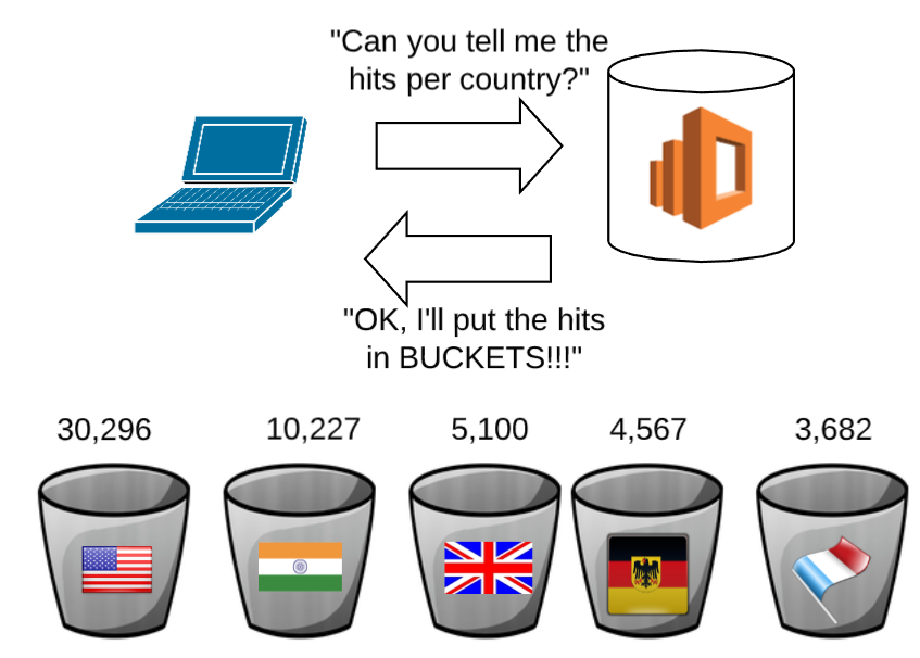
In Elasticsearch parlance, we put the rows into BUCKETS, with one BUCKET for each country. I use simple cartoons below to explain how BUCKETS work.
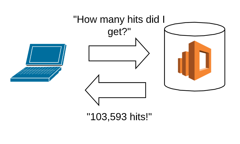
First, consider a query for total hits. The Elasticsearch API reports that I received ~100k hits in the month of June.
Our client uses the AGGS API to count the hits by country.
We now use the API to count the hits by day.
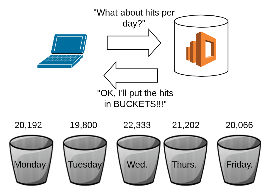
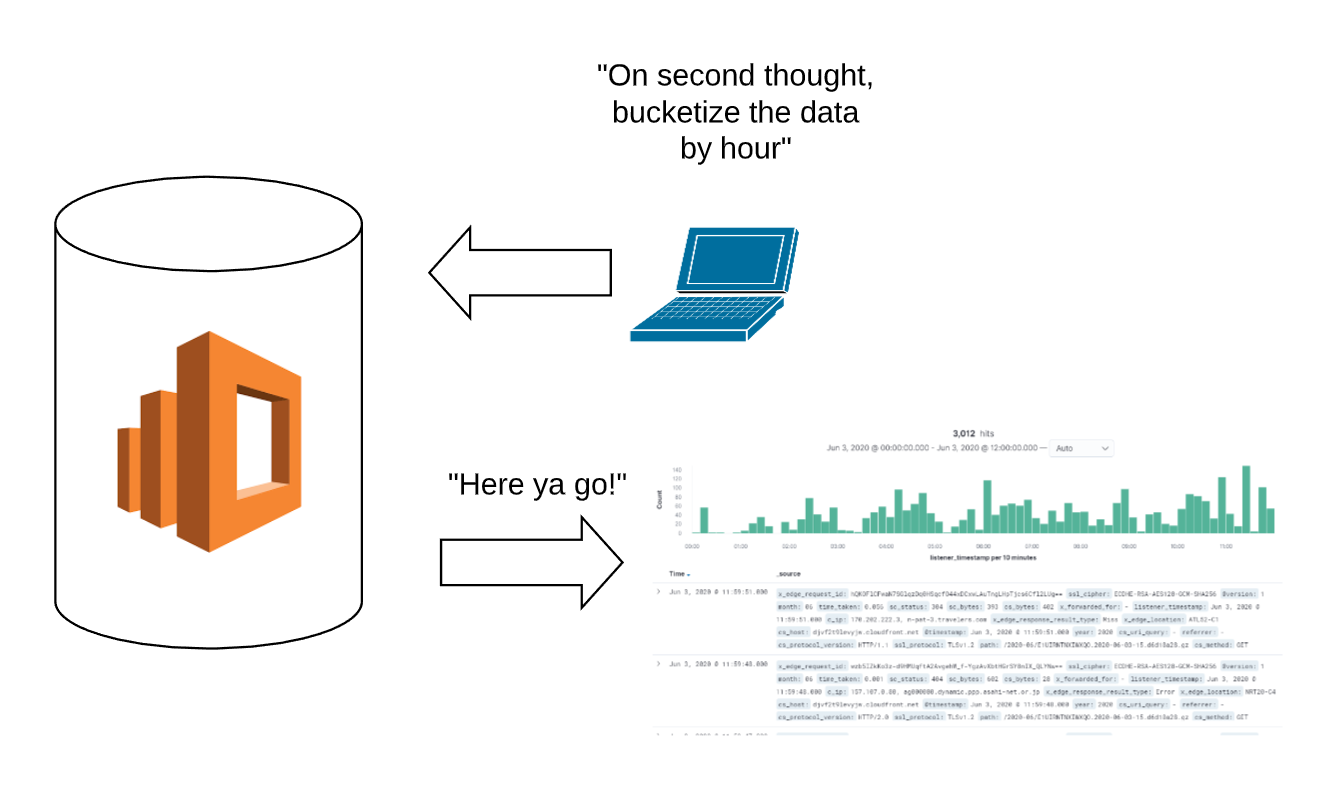
Time BUCKETS enable us to analyze, summarize and visualize time series data. We need BUCKETS because we cannot plot every datum from a big data document store.
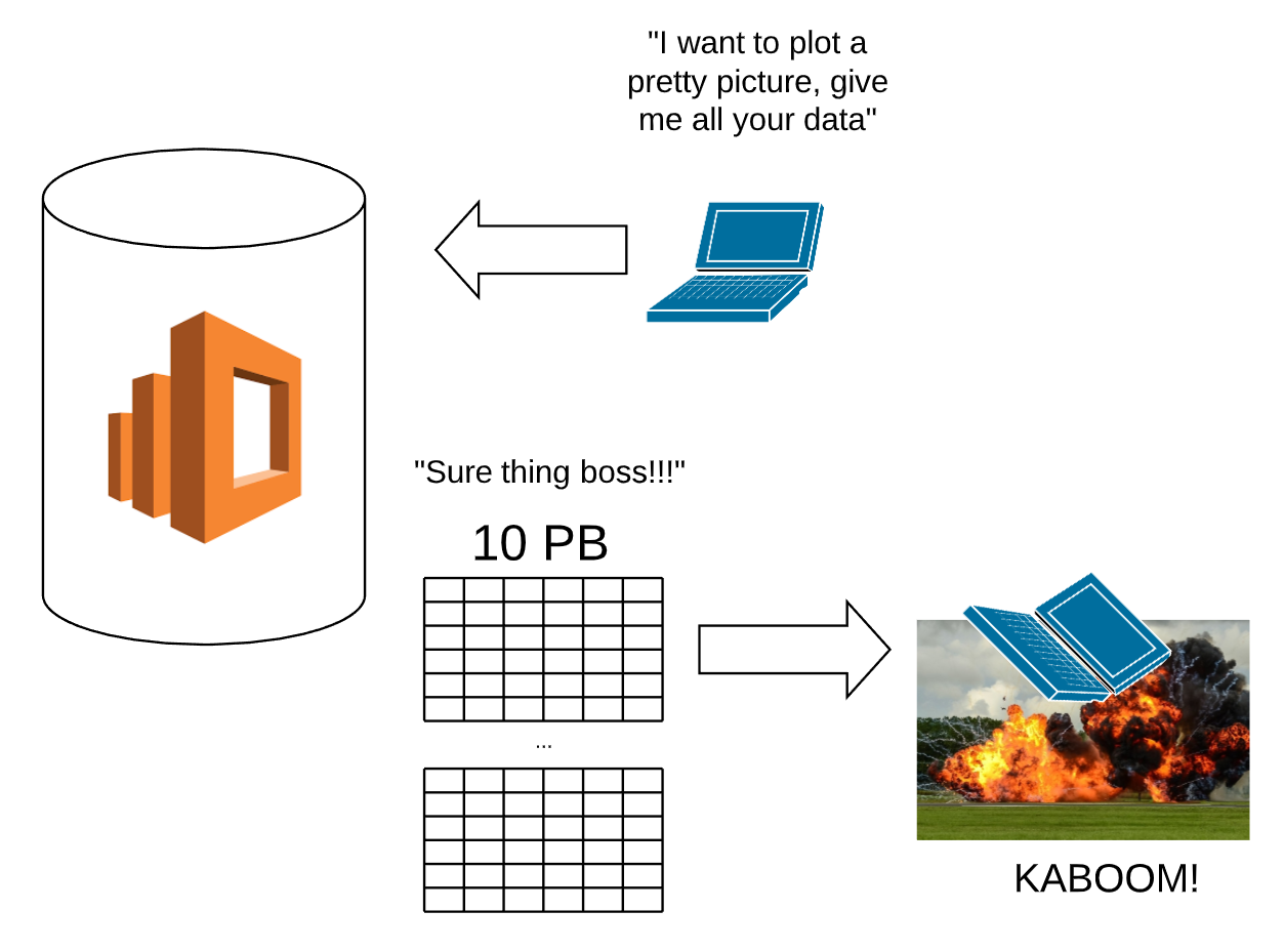
BUCKETS return a smaller amount of data, for example, hits per hour.
Time Series Data Viz with Kibana
I will demonstrate the idea of using BUCKETS for time series data viz through Kibana.
Simple Date Histogram
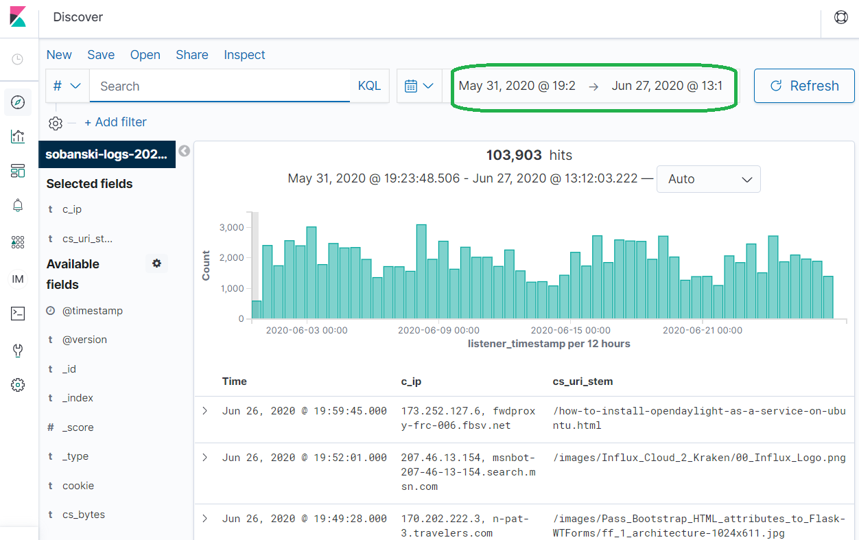
In the Kibana Discover panel, set the correct time range.
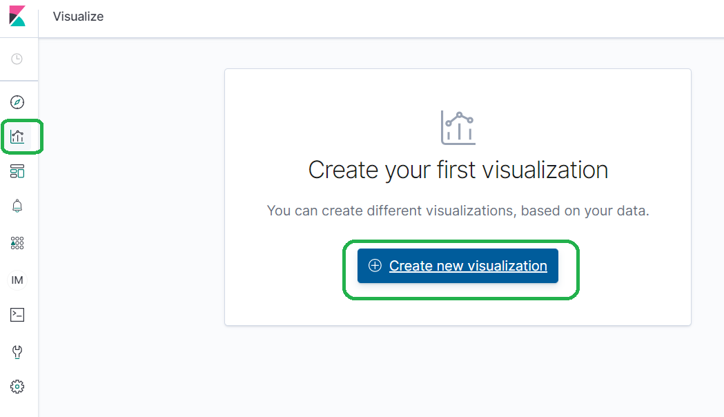
Click Visualization --> Create New Visualization
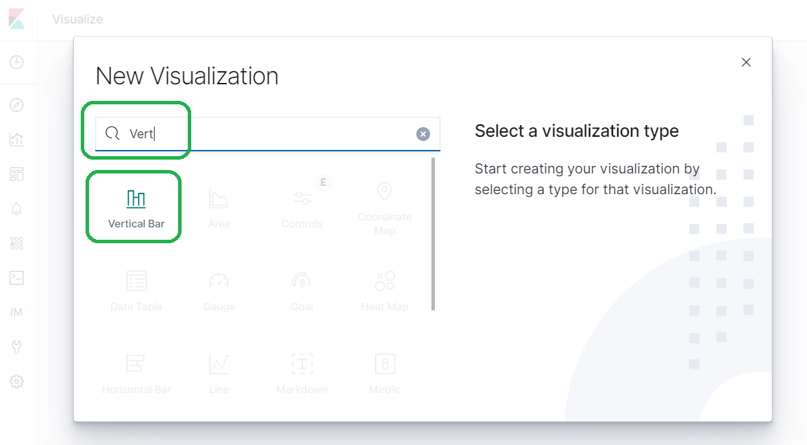
Type Vertical into the search bar and select Vertical Bar and then click the name of your index.
Elasticsearch uses Metric and Bucket parameters to drive AGGS. Leave Metrics to the default of Y-axis Count (this gives us hits), and expand Buckets. Click X-Axis.
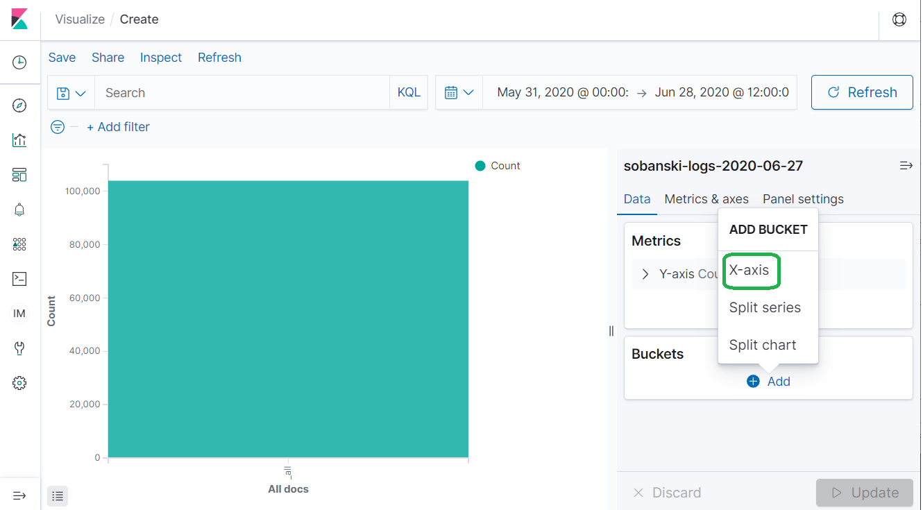
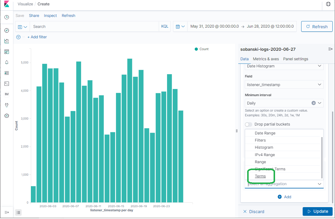
Now select Date Histogram and click Update.
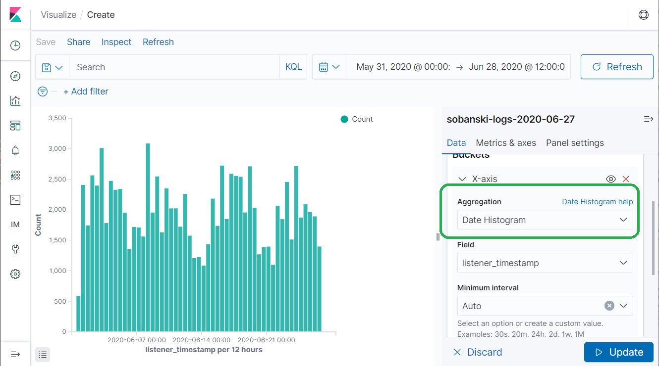
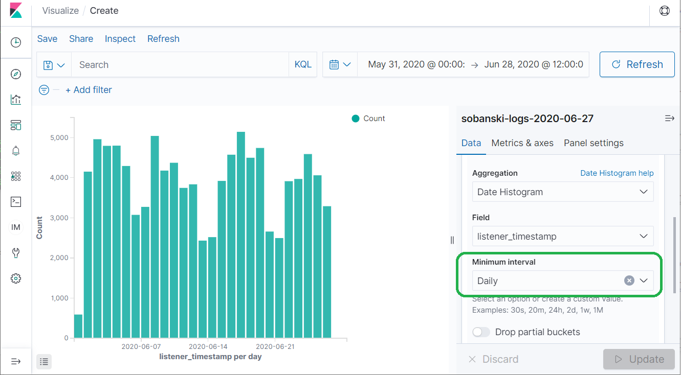
Elasticsearch placed the hits into time buckets for Kibana to display. Elasticsearch chose twelve hour buckets for the bucket size. Change minimum interval to Daily and Elasticsearch cuts the number of BUCKETS in half.
Nested Aggregation
In Aggregations - The Elasticsearch GROUP BY, I demonstrated how to chain, or nest AGGS together. Time Series data plays nicely with nested AGGS. The above diagram depicts hits per day. Use a Nested AGG to display hits per day broken down by country.
Under X-Axis, click Add and then Split Series.
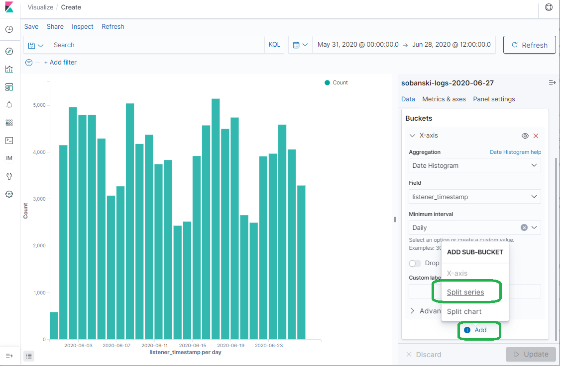
You want to split on the term Country, so select the TERMS sub aggregation.
Type country into the field pull-down and select geoip.country_name.keyword.
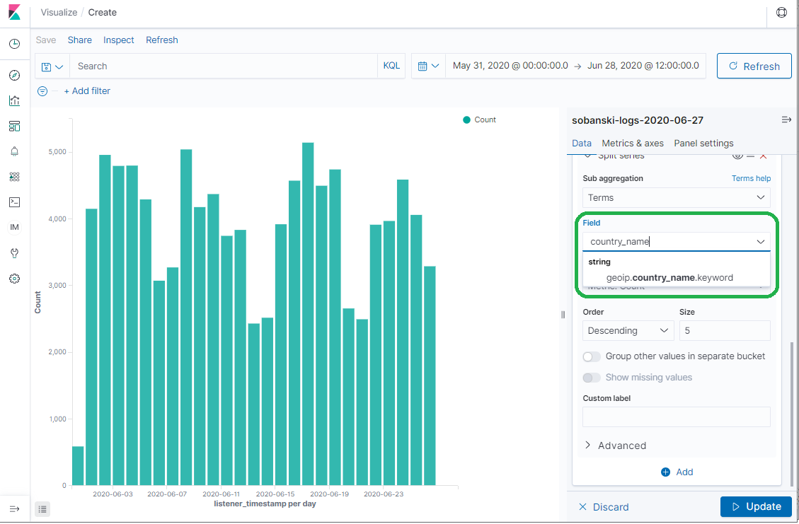
Click Update. Kibana presents the daily count by country.
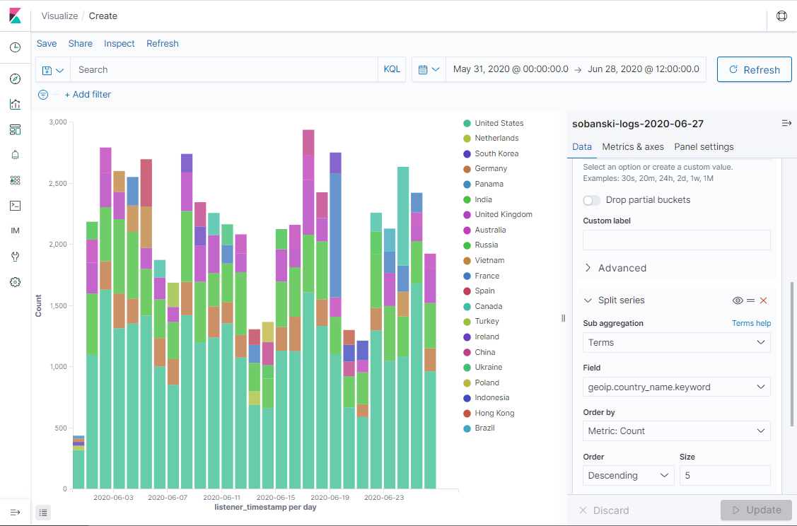
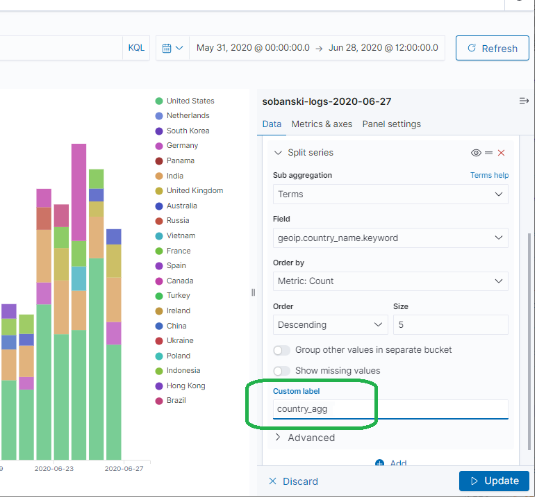
Name the Buckets
Bucket names will clear things up in the next section, when you use the Elasticsearch API to create buckets. First, give your parent bucket a name. In the Date Histogram Aggregation, set Custom Label to daily_agg.
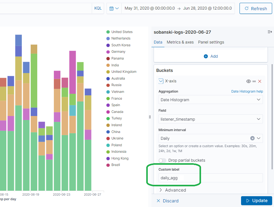
Under the Terms sub-aggregation, set Custom label to country_agg and click update.
Kibana Takeaway
Understand the key takeaways. We first created a Date Histogram aggregation (named daily_agg) on the listener_timestamp field. We then nested a Terms aggregation (named country_agg) on the field geoip.country_name.keyword. The sub-aggregation added child country buckets into each of the parent daily buckets.
Use the API
A good understanding of the terminology will help you navigate the API. If you do not feel comfortable with the terminology I encourage you to re-visit the first post in this series, Aggregations - The Elasticsearch GROUP BY.
The Kibana Dev Tools console allows you to drive the REST API. Dev Tools auto-completes your input. If you type the following into the console, Dev Tools will provide a popup with suggestions.
Note: Change sobanski-logs-2020-06-27 to the name your Cloudfront log index.
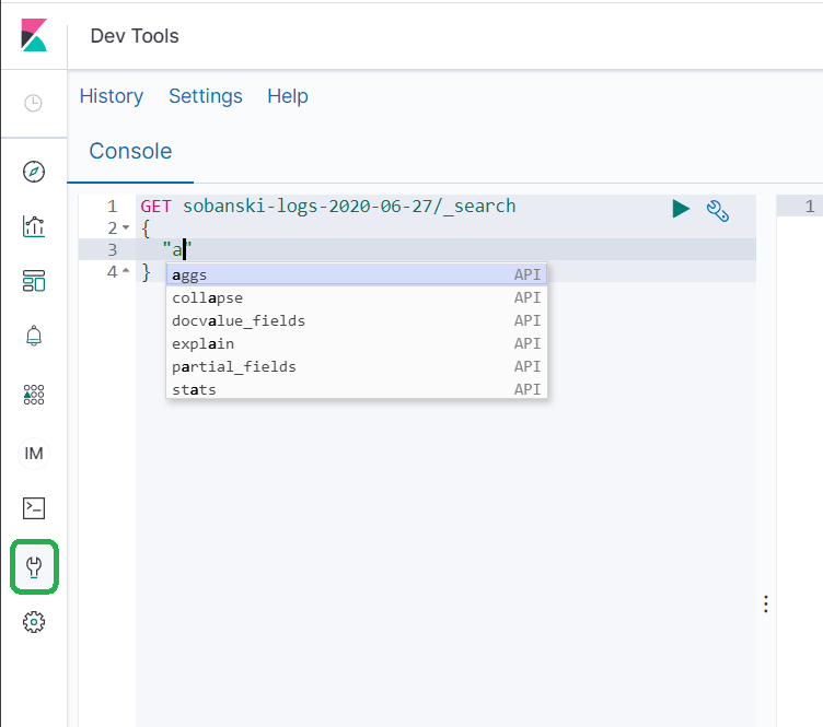
Select the aggs suggestion and Dev tools populates the Dev Tools console with the following JSON.
GET sobanski-logs-2020-06-27/_search
{
  "aggs": {
    "NAME": {
      "AGG_TYPE": {}
    }
  }
}
In the Kibana demonstration above, we first created a parent Date Histogram (named daily_agg) on the listener_timestamp field. In order to command the REST API to create a Date Histogram, first replace AGG_TYPE with date_histogram.
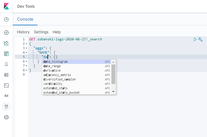
Dev Tools will auto-populate the JSON with the required date_histogram fields.
GET sobanski-logs-2020-06-27/_search
{
  "aggs": {
    "NAME": {
      "date_histogram": {
        "field": "date",
        "interval": "month"
      }
    }
  }
}
To match our Kibana visualization, set NAME to daily_agg, field to interval_timestamp and interval to day.
GET sobanski-logs-2020-06-27/_search
{
  "aggs": {
    "daily_agg": {
      "date_histogram": {
        "field": "listener_timestamp",
        "interval": "day"
      }
    }
  }
}
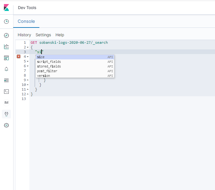
In addition, set size to zero, in order to filter out unwanted hits.
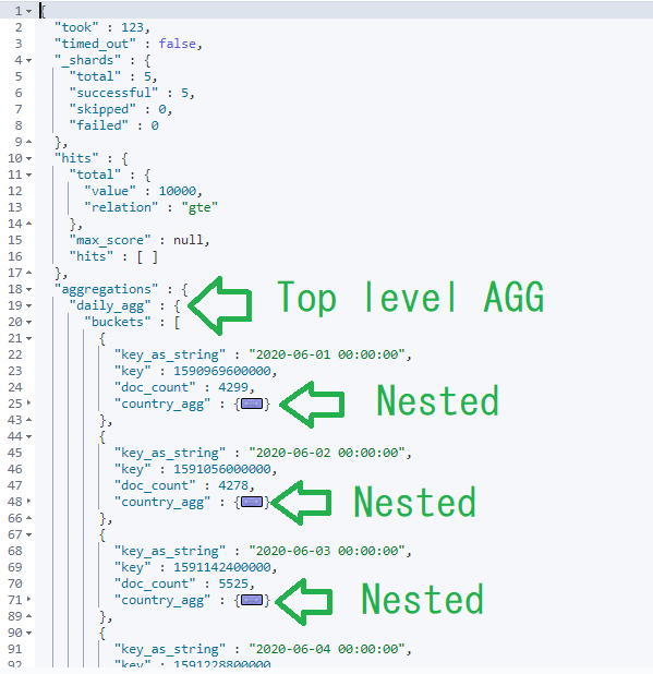
When you execute the script, Elasticsearch returns the JSON encoded results.
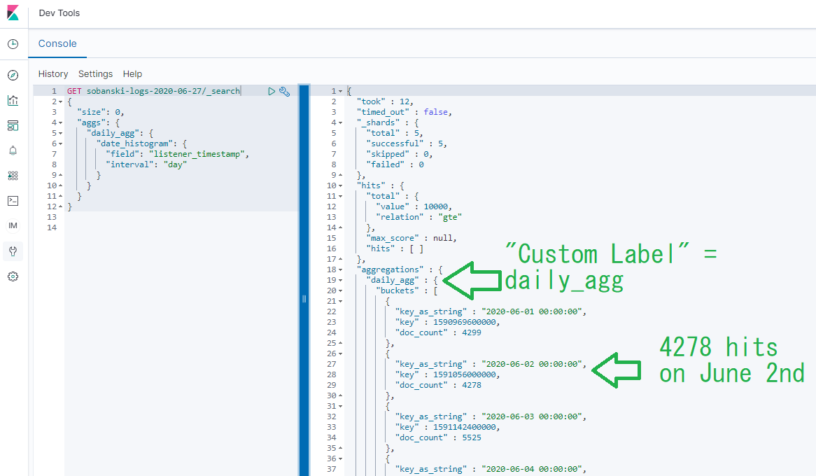
The daily_agg object contains an field named buckets, which contains an array of JSON objects. In this case, each bucket represents a day.
{
  "aggregations" : {
    "daily_agg" : {
      "buckets" : [
        {
          "key_as_string" : "2020-06-01 00:00:00",
          "key" : 1590969600000,
          "doc_count" : 4299
        },
        {
          "key_as_string" : "2020-06-02 00:00:00",
          "key" : 1591056000000,
          "doc_count" : 4278
        },
        {
          "key_as_string" : "2020-06-03 00:00:00",
          "key" : 1591142400000,
          "doc_count" : 5525
        }
      ]
    }
  }
}
In the Kibana example, we clicked the add button to add a sub aggregation. In this case we add a sub aggregation to the daily_agg object through a JSON stanza.
First, collapse the date_histogram object under the daily_agg object.
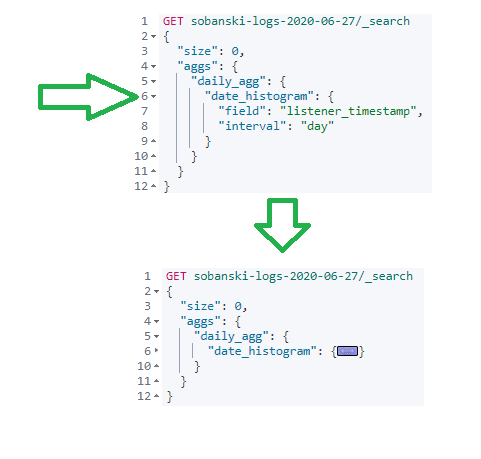
After date_histogram, add a comma and a quote followed by aggs. An auto-complete pop-up lets you know that you clicked the correct spot.
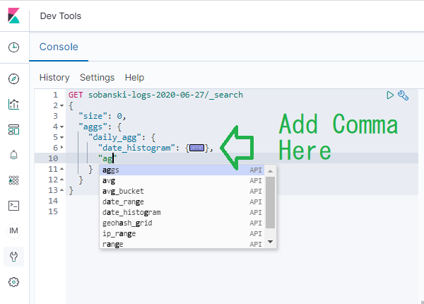
Note: No auto-complete means that you put the comma in the wrong spot.
Select AGGS from the pop-up.
GET sobanski-logs-2020-06-27/_search
{
  "size": 0,
  "aggs": {
    "daily_agg": {
      "date_histogram": {
        "field": "listener_timestamp",
        "interval": "day"
      },
      "aggs": {
        "NAME": {
          "AGG_TYPE": {}
        }
      }
    }
  }
}
Now, type terms into AGG_TYPE and click the pop-up.
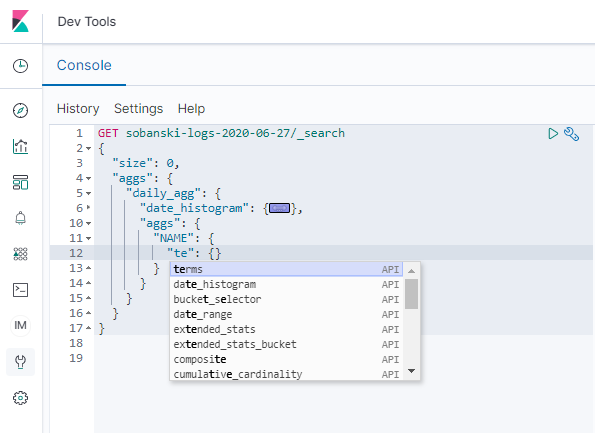
TERMS aggregations require a field (e.g. the GROUP_BY field). Begin to type city and the pop-up provides a list. Select geoip.city_name.keyword.
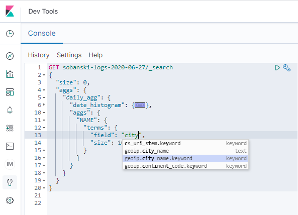
Set size to 3. Also, to match the Kibana example, set NAME to country_agg.
Your JSON should read:
GET sobanski-logs-2020-06-27/_search
{
  "size": 0,
  "aggs": {
    "daily_agg": {
      "date_histogram": {
        "field": "listener_timestamp",
        "interval": "day"
      },
      "aggs": {
        "country_agg": {
          "terms": {
            "field": "geoip.city_name.keyword",
            "size": 3
          }
        }
      }
    }
  }
}
Each day bucket in the daily_agg aggregation includes a nested country_agg.
Each nested country_agg object contains an field named buckets, which contains an array of JSON objects. In this case, each bucket represents a country. A zoom into Day 1, for example, reads:
{
  "country_agg" : {
    "buckets" : [
      {
        "key" : "Pune",
        "doc_count" : 112
      },
      {
        "key" : "Ashburn",
        "doc_count" : 94
      },
      {
        "key" : "Lisbon",
        "doc_count" : 73
      }
    ]
  }
}
The complete AGGS JSON for Days 1 and 2 reads:
{
  "aggregations" : {
    "daily_agg" : {
      "buckets" : [
        {
          "key_as_string" : "2020-06-01 00:00:00",
          "key" : 1590969600000,
          "doc_count" : 4299,
          "country_agg" : {
            "doc_count_error_upper_bound" : 45,
            "sum_other_doc_count" : 3057,
            "buckets" : [
              {
                "key" : "Pune",
                "doc_count" : 112
              },
              {
                "key" : "Ashburn",
                "doc_count" : 94
              },
              {
                "key" : "Lisbon",
                "doc_count" : 73
              }
            ]
          }
        },
        {
          "key_as_string" : "2020-06-02 00:00:00",
          "key" : 1591056000000,
          "doc_count" : 4278,
          "country_agg" : {
            "doc_count_error_upper_bound" : 47,
            "sum_other_doc_count" : 2948,
            "buckets" : [
              {
                "key" : "Ashburn",
                "doc_count" : 105
              },
              {
                "key" : "Raleigh",
                "doc_count" : 104
              },
              {
                "key" : "Pune",
                "doc_count" : 90
              }
            ]
          }
        }
       ]
    }
  }
}
The REST API returns the same data that the Kibana Data Viz returns, only in JSON format.
Conclusion
In this blog post I demonstrated how to use AGGS to visualize time series data. I also demonstrated how to use the Elasticsearch API to return time series data in JSON encoded format.