This blog post summarizes the first three chapters of Bernard Sklar's Digital Communication - Fundamentals and Applications textbook.
Signals
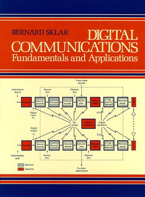
A Digital Communication System (DCS) transmitter (XMT) sends a waveform selected from a finite set of waveforms. A receiver (RCV) does not need to reproduce the waveform entirely, but only needs to determine from the degraded signal which waveform the signal best matches. The RCV regenerates digital signals with less effort and power than their analog counterparts.
Similar to computer networking’s seven layer Open System Interconnection (OSI) model, engineers break DCS into several discrete layers. Source Encoding, Encryption, Channel Encoding, Multiplexing, pulse modulation, bandpass modulation, frequency spreading and multiple access encompasses the signal transforms from the source to the XMT. The reverse path encompasses the signal transforms from the RCV to the sink. Most DCS convert data to a bit stream, which they convert to a voltage or current waveform with a pulse for baseband and sinusoid for bandpass XMT.
DCS include two types of signals, deterministic or random. Engineers use explicit mathematical expressions for deterministic signals, which they rarely use in real world communications. Engineers use stochastic or random processes to describe random signals using probability theory to characterize signals. Periodic signals repeat themselves over a finite period of time, and the period indicates time interval at which the signals start over. Continuous analog signals exist unbroken over time, whereas discrete signals exist only at discrete times. A roll of the die illustrates a discrete system, the outcome can only produce one of six predefined integers.
Engineers classify periodic and random signals power signals and classify deterministic and non periodic signals energy signals. The energy received by a RCV does the work, and power describes the rate at which the XMT delivers the energy. The Dirac delta, or unit impulse function helps with sifting or sampling random signal equations where a certain point may be equal to infinity.
Engineers characterize distribution of a signal's energy or power in the frequency domain through spectral density. Energy spectral density (ESD) sits symmetric in frequency about the origin and describes the signal energy per unit bandwidth measured in joules/ hertz. The power spectral density (PSD) provides a real, even, nonnegative, periodic function of frequency.
Autocorrelation measures how closely a signal matches a copy of itself through shifts in time. A real valued energy signal’s autocorrelation sits symmetric in time difference about zero, with a maximum value at zero. The autocorrelation and ESD form a Fourier transform pair. A real valued power signal shares the same properties, substituting in the fact that it forms a Fourier transform pair with its PSD.
Random Variables
Standard probability and statistics help define and characterize random signals, to include the probability density function (PDF), expected value, moment generating function and variance. Random or Stochastic processes collect N sample Random Variables over time, all of which we refer call an ensemble.
Strict sense stationary random processes witness no statistics change with a shift in the time origin. Wide sense stationary (WSS) processes witness no change to their mean and autocorrelation. Variance gives a sense of randomness for a random variable. Autocorrelation does the same for a random process.
If a random process's autocorrelation changes slowly upon approach of the autocorrelation time difference number, then the frequency domain representation will show mostly low frequencies. If the autocorrelation changes quickly, we can expect to see mostly high frequencies. Ergodic random processes have equal time and ensemble averages and therefore, engineers can determine the statistical properties by time averaging over a single sample function of the process.
A power signal (random process) describes the distribution of power in the frequency domain using a PSD. The PSD will record a reading greater than zero, sit symmetric around zero, and forms a Fourier transform pair with autocorrelation. We can look at the width of the main spectral lobe of the PSD to measure bandwidth. The central limit theorem states that the pdf of the sum of j independent random variables approaches Gaussian distribution as j approaches infinity. Engineers, therefore use zero mean Gaussian normal pdf to describe thermal noise. Engineers use additive white Gaussian noise (AWGN) in models to corrupt signal systems.
Engineers can use signals in either the time or frequency domain to characterize the effects of systems on signals. The impulse response characterizes the system in the time domain. Taking a Fourier transform of the time domain equations yields the frequency domain equations. The Fourier transform of the impulse response function yields the frequency transfer function, or the frequency response. If a random process forms the input to a time-invariant linear system, the output will also yield a random process.
A distortionless transmission medium can never be created, since it requires infinite bandwidth. Engineers can attain an ideal filter through minimum and maximum cutoff frequencies. A zero minimum cutoff frequency and a finite maximum cutoff frequency produces a low pass filter. A non-zero minimum cutoff frequency combined with a finite maximum cutoff frequency produces a bandpass filter. A filter with a non zero minimum cutoff frequency combined with a maximum cutoff frequency that approaches infinity produces a high pass filter.
Digital Messages
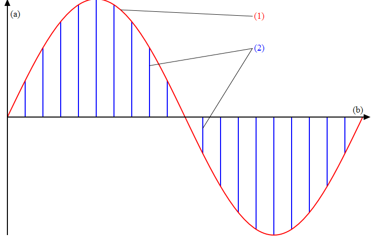
XMT transform information into digital messages, and pulse modulate the messages into baseband waveforms. A baseband signal's spectrum extends from (or near) dc to some finite value, usually less than a few megahertz (MHz). Coaxial cable provides an example baseband channel. Engineers format an analog waveform into a form compatible with DCS through sampling, with sample and hold the most popular method. A transistor and capacitor, for example, sample an incoming analog signal and output pulse amplitude modulation (PAM). Engineers then use low pass filtering to retrieve the original analog waveform.
The sampling theorem states that a bandlimited signal having no spectral components above fm hertz can be determined uniquely from a sampling rate of fs >= 2 fm, the Nyquist rate. Aliasing refers to lost information due to undersampling. Higher sample rates eliminate aliasing by separating the spectral replicates.
Antialiasing filters, either pre or post filtering provide a way to remove aliasing. Prefiltering reduces the maximum frequency, and thus the Nyquist criterion. Postfiltering removes the aliased components. Both filtering techniques result in some signal loss, and thus sample rate. In order to increase the transition bandwidth, engineers have modified the Nyquist criterion to the Engineer’s criterion, that fs >= 2.2 fm.
For compatibility with a DCS, the Pulse Amplitude Modulation (PAM) levels must be of a finite number of predetermined levels or quantized samples. Some sources of corruption occur during quantization, since the system converts the infinite continuous analog levels into a finite number of predefined levels. The step sizes between a quantization levels are called quantile intervals, which we denote q volts. Quantization levels can be uniform or linear, but more often nonuniform, to reflect the statistical distributions of peak to peak levels. The error due to the quantization approximation error registers no more than +/-q/2 volts in either direction or 2 quantile intervals. If you a uniform distribution of quantization error over a quantile interval, you can use probability theory to describe the variance, or average quantization noise power.
From this, and the number of quantization levels, you can describe the peak power of the analog signal. S/N or 3L2 represents the ratio of peak signal power to average quantization noise power (variance)..
Pulse code modulation (PCM) represents the act of encoding each quantized PAM sample into a class of baseband signals through a digital word. The MXT samples the source information and quantized it into one of L levels and then digitally encodes each quantized sample into a bit word.
For baseband transmission, the XMT transforms these words into pulse waveforms. PCM encompass numerous types and each have different levels of efficiency in using bandwidth. hertz/symbols notes the spectral attributes of PCM waveforms . A PCM waveform that uses more than 1 hertz per symbol yields less efficiency than one that uses less than 1. In order to define the PCM word size, we use the formula 1 >= log2(1/2p) bits, with p equal to the acceptable quantization distortion, which indicates the percentage of the peak-to-peak analog signal.
Equalization
Equalization refers to any signal processing or filtering technique that eliminates or reduces Intersymbol Interference (ISI). ISI captures the overlap or smearing that distorts a transmitted sequence of pulses. A communication channel needs a constant amplitude response, or the channel distorts a signal’s amplitude. A channel needs a linear function of frequency for phase response, or the channel distorts phase. Equalization includes two broad categories: Maximum Likelihood sequence estimation (MLSE) and Equalization with filters, which we further categorize into transversal or decision feedback, preset or adaptive and symbol or fractionally spaced.
MLSE measures impulse response and then adjusts the receiver to allow the detector to make good estimates from the demodulated distorted pulse sequence. The MLSE receiver does not reshape or compensate for the distorted signals, instead, it adjusts itself to better deal with the distorted samples.
An ideal Nyquist filter ensures the ISI is zero at sampling points. The H(f) raised cosine filter transfer function belongs to the Nyquist. The cosine filter's roll off factor represents the fractional excess bandwidth. A value of one yields 100% excess bandwidth, and zero would be the Nyquist minimum bandwidth case. Eye patterns can help identify ISI. A “closing eye” signals increasing ISI, and “opening eye” signals less.
A transversal equalizer filter consists of a delay line with T-second taps, and T records the symbol duration. The DCS linearly weights the current and past values of the received signal with tap weights and sum these weights to produce outputs. The DCS amplifies, sums and feeds the outputs of the taps to a coefficient adjustment device. An engineer chooses the tap weights to subtract the interference effects from symbols adjacent in time to the desired symbol. A zero forcing equalizer forces the equalizer output on either side of the desired pulse. The introduced channel smearing drives the outputs of the taps. A Minimum mean square error (MSE) equalizer engineer chooses tap weights to minimize MSE of all the ISI terms and the noise power at the output of the equalizer. MSE represents the expected value of the squared difference between the desired symbol and the estimated symbol. Designers of this filter send a known test signal over a channel and use time averaging to solve for tap weights.
Engineers call a non-linear equalizer that uses previous detector decisions to eliminate ISI on pulses during demodulation a decision feedback estimator (DFE). The detector output provides an additional filter on t and recursively feeds a signal back to the detector input, to help it adjust tap weights.
Preset equalization use fixed tap weights during data transmission, whether decided mathematically, or after an initial training test. Preset equalization sets tap weights once at the start of transmission. Adaptive equalization, however, performs tap weight adjustments either continually or periodically. In the decision directed method, an XMT sends a periodic preamble, which allows the receiver to adjust its tap weights accordingly.