The discipline of Operations Research (OR) applies analytical methods from math, statistics, economics, and computer science to help leaders make good decisions.
Enterprise software consumes physical resources (CPU, Memory, Disk, and Bandwidth) to provide mission-essential services. Software, Cloud, and Data Center Architects must identify the expected resource consumption to optimize resource spend. Operations Research Engineers develop Capacity Planning models to drive decisions around CAPEX and OPEX purchases.
Today you will learn how to develop a Python Pandas Capacity Planning model that right sizes the resources needed for a simple Web Application.
Approach
We use concepts from Fermi Estimation and the Jackson Network Theorem (Product-Form Solution) to drive our model. Both allow us to remove unnecessary details (and rabbit holes) from our model. Our model will nonetheless yield a reasonable estimate.
BONUS: Our approach yields artifacts (flow diagrams) that demonstrate rigorous, considerate thought and discipline. You can expect them to satisfy (most) audits or engineering reviews.
The stages of our model development workflow include:
- Record the Nominal Architecture (Node Diagram)
- ID the Data Flows through the Architecture (Use Cases)
- Estimate the Maximum Throughput per flow (Gb/s)
- Sum the Max Throughput for Each Node
- Map Max Gb/s to the required number of CPUs per Node
- Price the Sum Total for the required CPUs ($)
1. Record the Nominal Architecture (Node Diagram)
For illustration, we will size a simple web application. The set of Application Nodes includes an App Server, File Store, Firewall, and a Core Switch that connects the nodes. Users and Developers both use the system.
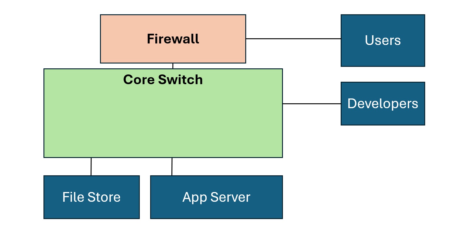
NOTE: Once you understand our approach, feel free to tailor the names and roles of the Nodes for your models.
2. ID the Data Flows through the Architecture (Use Cases)
Our Application hosts a Photo Album service. Users upload and retrieve photos via the Web Application. Developers look at logs from the server to optimize the user experience.
The following graphic captures the three main flows.
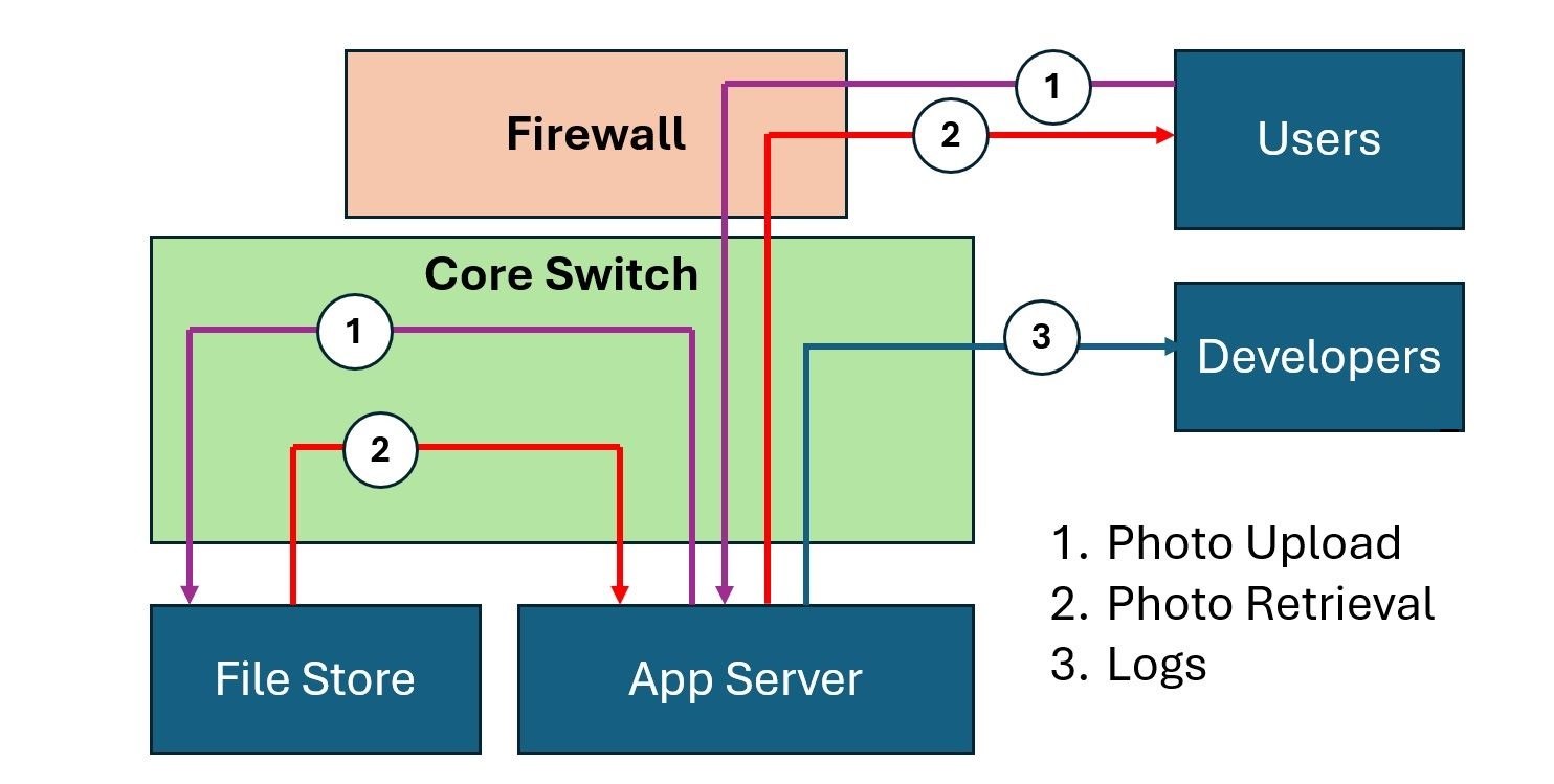
The Three Flows include:
- Photo upload
- Photo Retrieval
- Logs
3. Estimate the Maximum Throughput per flow (Gb/s)
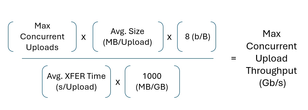
How do we estimate the expected throughput of our system? File Size, Upload Time, and (Max) Number of Concurrent Users drive the throughput.
The following model produces the desired metric:
For example, assume that each photo averages four (4) MegaBytes (MB) in size. My Samsung Galaxy phone produces photos of this size by default. Then, assume we have (at max) thirty-two (32) Concurrent Users and each photo takes 1/4 a second to upload.
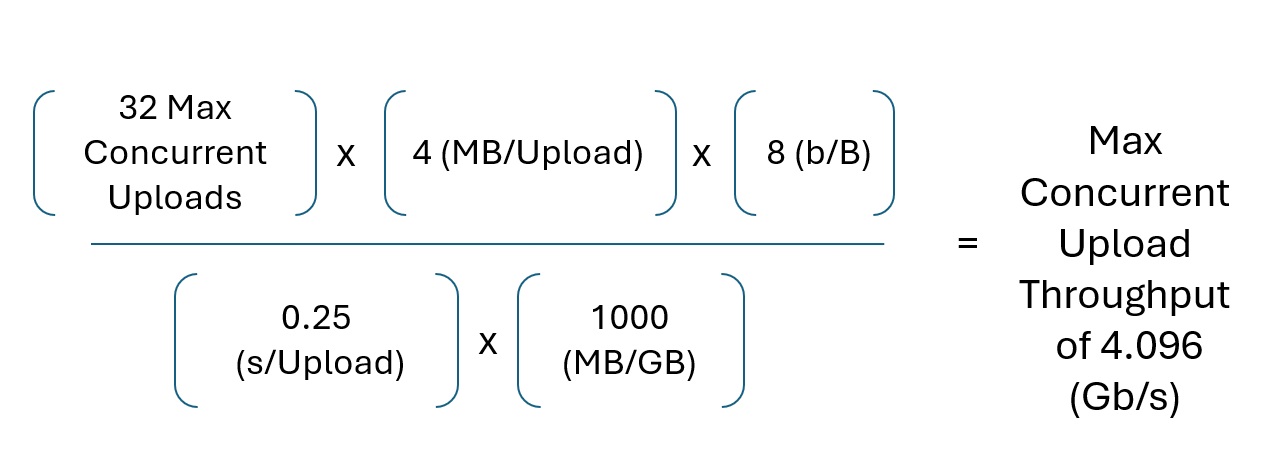
This formula estimates a max throughput of four (4) Gigabits per second (Gb/s) for our file upload use case.
Another formula calculates the logs' maximum network capacity consumption.
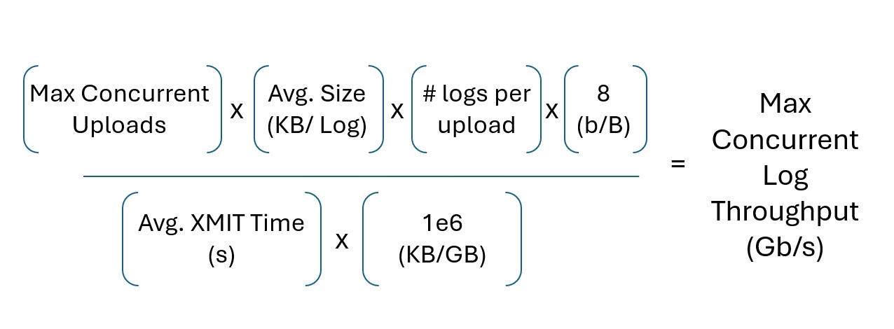
An average Syslog (for Apache2) yields about one and a half (1.5) KiloBytes (KB).
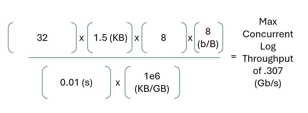
This formula yields a max of 0.307 Gb/s for log traffic.
Feel free to either benchmark your data or use rough order of magnitude (ROM) numbers in your calculation. When you run the model, you will learn that ROM numbers provide enough data for acceptible results.
4. Sum the Max Throughput for Each Node
This stage of our pipeline uses code from the Python Pandas and Numpy libraries.
import pandas as pd
import numpy as np
Map Flows to Tables
We need to map our data flows from our flow diagram to a Pandas DataFrame.
In the flow above, we see that the Photo Upload Flow originates at the User, hits the Firewall, traverses the Core Switch to the App Server, and then terminates at the File Store via another trip through the Core Switch.
We map this description to the following table:
| Flow | Data | SourceNode | DestinationNode |
|---|---|---|---|
| 1 | photo_upload | user | firewall |
| 1 | photo_upload | firewall | core_switch |
| 1 | photo_upload | core_switch | app_server |
| 1 | photo_upload | app_server | core_switch |
| 1 | photo_upload | core_switch | file_store |
We can ignore the User to Firewall flow since we do not want to size the User's computer.
To further minimize rote work, we will delete the Core Switch entries. Since every flow navigates through the core switch, we will add those in one batch job at a later point.
We reduce the above table to:
| Flow | Data | SourceNode | DestinationNode |
|---|---|---|---|
| 1 | photo_upload | firewall | app_server |
| 1 | photo_upload | app_server | file_store |
We append the photo_retrieval and logs flows to the table.
| Flow | Data | SourceNode | DestinationNode |
|---|---|---|---|
| 1 | photo_upload | firewall | app_server |
| 1 | photo_upload | app_server | file_store |
| 2 | photo_retrieval | file_store | app_server |
| 2 | photo_retrieval | app_server | firewall |
| 3 | logs | app_server | developers |
We use a Python Dict to import the data. You can also use a Comma Separated Variable (CSV) file, a Structured Query Language (SQL) table, or JavaScript Object Notation (JSON) to encode your flows.
flow = {'Data': ['photo_upload',
  'photo_upload',
  'photo_retrieval',
  'photo_retrieval',
  'logs'],
 'SourceNode': ['firewall',
  'app_server',
  'file_store',
  'app_server',
  'app_server'],
 'DestinationNode': ['app_server',
  'file_store',
  'app_server',
  'firewall',
  'developers']}
We then import the Dict into a Pandas DataFrame.
Flow = pd.DataFrame(data=flow)
Print displays the Flow DataFrame.
print(Flow)

    ...

              Data  SourceNode DestinationNode
0     photo_upload    firewall      app_server
1     photo_upload  app_server      file_store
2  photo_retrieval  file_store      app_server
3  photo_retrieval  app_server        firewall
4             logs  app_server      developers
NOTE: You can add more rows and flows to suit your needs.
We now add the Core Switch nodes back into the table.
Core_Flows = (pd
              .concat([Flow
                       .copy()
                       .assign(DestinationNode='core_switch'),
                       Flow
                       .copy()
                       .assign(SourceNode='core_switch')],
                      ignore_index=True))
This batch job introduces the Core Switch back into the flows.
print(Core_Flows)

              Data   SourceNode DestinationNode
0     photo_upload     firewall     core_switch
1     photo_upload   app_server     core_switch
2  photo_retrieval   file_store     core_switch
3  photo_retrieval   app_server     core_switch
4             logs   app_server     core_switch
5     photo_upload  core_switch      app_server
6     photo_upload  core_switch      file_store
7  photo_retrieval  core_switch      app_server
8  photo_retrieval  core_switch        firewall
9             logs  core_switch      developers
NOTE: The above code outputs an arbitrary ordering of the flows. We can ignore the order since we aim to execute a per-node GROUP BY operation at the end of our pipeline.
Our model requires a Node view of the flows, independent of Source or Destination.
We achieve this through the following Pandas operations:
Node_Flows = (pd
 .concat([Core_Flows
          .drop('DestinationNode',
                axis=1)
          .rename(columns={'SourceNode': 'Node'}),
          Core_Flows.drop('SourceNode', axis=1)
          .rename(columns={'DestinationNode': 'Node'})]
         ,ignore_index=True))
Our concat operation outputs:
print(Node_Flows.sort_values('Node', ignore_index= True))

   ...

]
0s
print(Node_Flows.sort_values('Node', ignore_index= True))

               Data         Node
0      photo_upload   app_server
1   photo_retrieval   app_server
2   photo_retrieval   app_server
3              logs   app_server
4      photo_upload   app_server
5              logs  core_switch
6      photo_upload  core_switch
7      photo_upload  core_switch
8   photo_retrieval  core_switch
9   photo_retrieval  core_switch
10     photo_upload  core_switch
11     photo_upload  core_switch
12  photo_retrieval  core_switch
13  photo_retrieval  core_switch
14             logs  core_switch
15             logs   developers
16     photo_upload   file_store
17  photo_retrieval   file_store
18  photo_retrieval     firewall
19     photo_upload     firewall
A simple GROUP BY operation verifies the quantity of Flows per Node. The Output of the operation matches the number of Flows per Node in our Flow Diagram.
print(Node_Flows
      .groupby('Node')['Data'].count())

    ...

Node
app_server      8
core_switch    16
developers      1
file_store      4
firewall        3
Name: Data, dtype: int64
JOIN Data Rates into Node Flow Table
I use another Dict to import the (Estimated) Max Throughput for the Upload, Retrieval, and Logs data flows into a DataFrame. Once more, you can use the encoding format of your choosing (CSV, SQL, JSON).
data = {'Data': ['photo_upload',
                 'photo_retrieval',
                 'logs'],
        'RateGbps': [4.096,
                     4.096,
                     0.307,]}

Data = pd.DataFrame(data=data)
This yields:
print(Data)

    ...

              Data  RateGbps
0     photo_upload     4.096
1  photo_retrieval     4.096
2             logs     0.307
We JOIN this Data DataFrame into our Flow DataFrame via a merge operation.
We also apply a SUM operation via the GROUP BY method.
# prompt: join Node_Flows and Data on Data

Node_Flows_Data = (pd
                   .merge(Node_Flows,
                          Data,
                          on='Data',
                          how='left')
                   .groupby('Node')['RateGbps']
                   .sum()
                   .reset_index())
This then outputs the MAX throughput (sum of ALL flows) on a per-node basis.
print(Node_Flows_Data)

    ...

          Node  RateGbps
0   app_server    18.341
1  core_switch    36.682
2   developers     0.307
3   file_store     9.292
4     firewall     8.742
5. Map Max Gb/s to the required number of CPU per Node
Assume that each CPU's cycle per second can process one bit of throughput, or one bit per Hertz (Hz).
We identify the number of cores needed via this calculation.
For purposes of this model, I use the Intel Xeon Silver 4214 Processor which retails at approximately $185.00 (USD) in 2024.
We feed our model with the Silver's specs (2.2GHz, 12C, 16.5MB Cache):
CPU_NAME = 'Intel Xeon Silver 4214'
CPU_CLOCK_SPEED = 2.2
CPU_CORES = 12
CPU_PRICE = 185.00
In addition, we need to account for various processing overhead, or Taxes. Feel free to benchmark your metrics. I use the following percentages:
OS_TAX = 0.05
VIRTUALIZATION_TAX = 0.15
TLS_TAX = 0.05
From here, we convert the Max Gb/s per node to Ghz to Cores. Note the Ceiling operation, since we can't buy a fractional core:
Node_Flows_Data['NumCores'] = (np
                               .ceil(Node_Flows_Data['RateGbps']
                                     *(1
                                       + OS_TAX
                                       + VIRTUALIZATION_TAX
                                       + TLS_TAX)
                                     /(CPU_CLOCK_SPEED)))
Based on the above math, we see that the core_switch requires the most cores:
          Node  RateGbps  NumCores
0   app_server    18.341      11.0
1  core_switch    36.682      21.0
2   developers     0.307       1.0
3   file_store     9.292       6.0
4     firewall     8.742       5.0
6. Price the Sum Total for the required CPU ($)
We know that each CPU includes twelve (12) 2.66 GHz cores and costs $185 per CPU. We use the following Pandas statements to calculate the cost.
Node_Flows_Data['NumCpu'] = (np
                             .ceil(Node_Flows_Data['NumCores']
                                   /CPU_CORES))

Node_Flows_Data['TotalCpuCost'] = (Node_Flows_Data['NumCpu']
                                *CPU_PRICE)
The following lines of code add a Totals row:
Total_Row = (Node_Flows_Data
             .sum(numeric_only=True))

Total_Row['Node'] = 'Total'

Node_Flows_Data = (pd
                   .concat([Node_Flows_Data,
                            pd
                              .DataFrame([Total_Row])],
                            ignore_index=True))
The final output Reads:
print(Node_Flows_Data)

    ...

          Node  RateGbps  NumCores  NumCpu  TotalCpuCost
0   app_server    16.691      10.0     1.0         185.0
1  core_switch    33.382      19.0     2.0         370.0
2   developers     0.307       1.0     1.0         185.0
3   file_store     8.192       5.0     1.0         185.0
4     firewall     8.192       5.0     1.0         185.0
5        Total    66.764      40.0     6.0        1110.0
We can expect to pay $1,100 to purchase the required CPU for our Photo Album Web Application.
Bonus: Extend the model
We can easily add new flows to our model.
For example, let's add a Data Analyst use case to our system. The Data Analysts look at new Metadata Flows (Flows four and five in the diagram below):
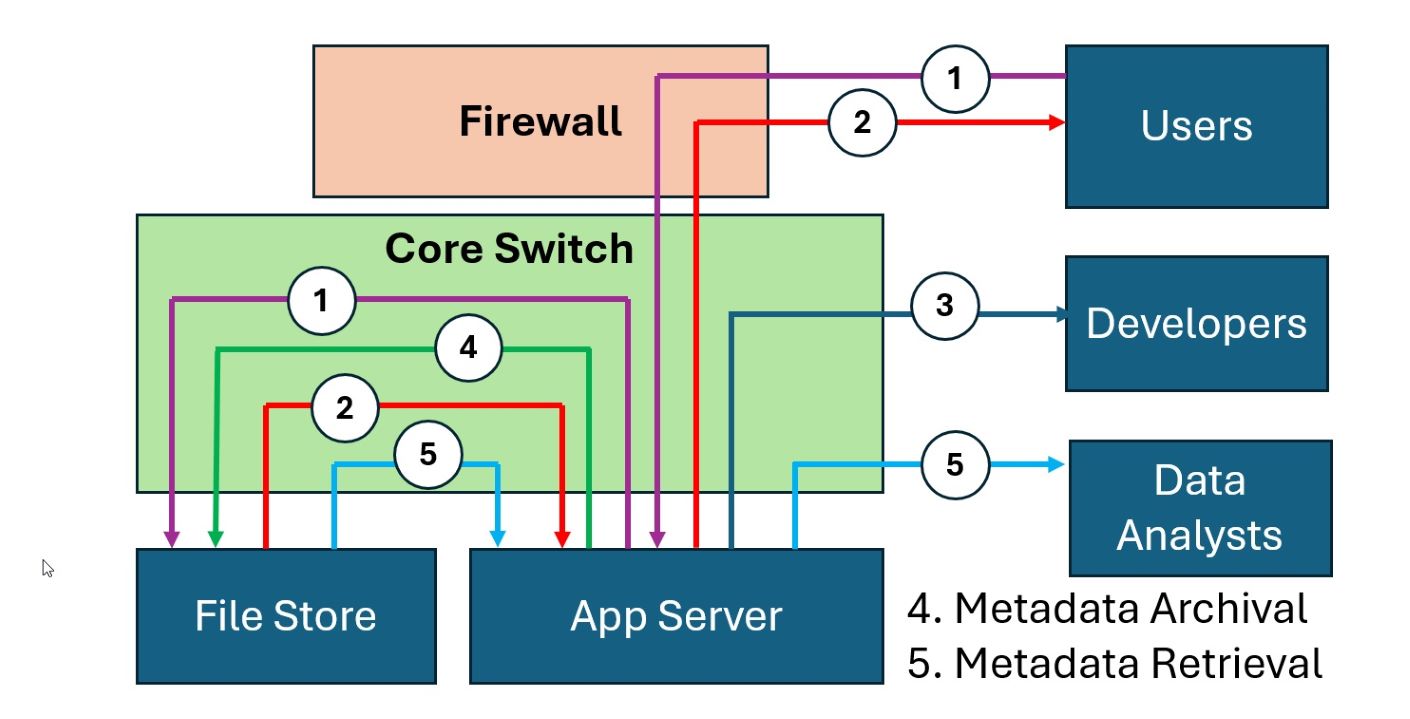
We add these two new flows (From the App Server to the File Store, and from the File Store to the Analysts) to our Flow and Data DataFrames:
flow = {'Data': ['photo_upload',
  'photo_upload',
  'photo_retrieval',
  'photo_retrieval',
  'logs',
  'metadata_archival',
  'metadata_retrieval',
  'metadata_retrieval',],
 'SourceNode': ['firewall',
  'app_server',
  'file_store',
  'app_server',
  'app_server',
  'app_server',
  'file_store',
  'app_server',],
 'DestinationNode': ['app_server',
  'file_store',
  'app_server',
  'firewall',
  'developers',
  'file_store',
  'app_server',
  'data_analysts',]}

Flow = pd.DataFrame(data=flow)
The Flow DataFrame now includes Metadata flows:
print(Flow)

    ...

                 Data  SourceNode DestinationNode
0        photo_upload    firewall      app_server
1        photo_upload  app_server      file_store
2     photo_retrieval  file_store      app_server
3     photo_retrieval  app_server        firewall
4                logs  app_server      developers
5   metadata_archival  app_server      file_store
6  metadata_retrieval  file_store      app_server
7  metadata_retrieval  app_server   data_analysts
We also update the Data DataFrame to include Metadata flows:
data = {'Data': ['photo_upload',
                 'photo_retrieval',
                 'logs',
                 'metadata_archival',
                 'metadata_retrieval'],
        'RateGbps': [4.096,
                     4.096,
                     0.307,
                     0.550,
                     0.550]}

Data = pd.DataFrame(data=data)
We then run the rest of the commands above, without edit, and the model learns about the new Node (Analysts) and Flows (Metadata Archival & Retrieval).
We see that we only need to buy one (1) new CPU for the Data Analyst's workstation:
            Node  RateGbps  NumCores  NumCpu  TotalCpuCost
0     app_server    18.341      11.0     1.0         185.0
1    core_switch    36.682      21.0     2.0         370.0
2  data_analysts     0.550       1.0     1.0         185.0
3     developers     0.307       1.0     1.0         185.0
4     file_store     9.292       6.0     1.0         185.0
5       firewall     8.192       5.0     1.0         185.0
6          Total    73.364      45.0     7.0        1295.0